Model and source
- Citation: Gao L, Xu H, Ye Q, Li S, Wang J, Mei Y, Niu C, Kang T, Chen C, Wang Y. Population Pharmacokinetics and Dosage Optimization of Teicoplanin in Children With Different Renal Functions. Front Pharmacol. 2020;11:552. doi:10.3389/fphar.2020.00552
- Description: Two-compartment IV-infusion population PK model for teicoplanin in 136 Chinese children aged 0.17-9.42 years with different renal functions (Gao 2020). Central volume scales with natural-log body weight, (ln(WT)/2.3)^0.14; peripheral volume with (WT/10)^0.19; clearance with (WT/10)^0.74 and modified-Schwartz eGFR (eGFR/118.99)^0.60. Inter-compartmental clearance has no covariate. Power residual error model with exponent 0.5.
- Article: Front Pharmacol 2020;11:552
Population
Gao 2020 enrolled 136 Chinese children (79 male, 57 female) aged 0.17-9.42 years with Gram-positive infections at Wuhan Children’s Hospital between February 2016 and January 2019. Median body weight was 10 kg (range 3.5-38), median age 1.25 years, and median modified-Schwartz eGFR 118.99 mL/min/1.73 m^2 (range 30.09-280). By renal function, 42 children had augmented function (eGFR >= 130), 63 normal (90-130), 23 mild insufficiency (60-90) and 8 moderate insufficiency (30-60). There were no neonates; the youngest patient was 2 months old. Teicoplanin was given as an IV infusion, three loading doses of 10 mg/kg every 12 h followed by 10 mg/kg once daily. 155 serum concentrations (1-3 per child, 150 at steady state) were analysed (Gao 2020 Table 1 and Results).
The same information is available programmatically via
readModelDb("Gao_2020_teicoplanin")$population.
Source trace
| Equation / parameter | Value | Source location |
|---|---|---|
| Two-compartment, first-order elimination | n/a | Results, “two-compartment model with first-order elimination” |
lvc (V1) |
2.31 L | Table 4, theta V1 |
lvp (V2) |
16.19 L | Table 4, theta V2 |
lcl (CL) |
0.13 L/h | Table 4, theta CL |
lq (Q) |
0.23 L/h | Table 4, theta Q |
e_lnwt_vc |
0.14 | Table 4, theta 1; Eq. 15
V1 = thetaV1 * (lnWT/2.3)^theta1
|
e_wt_vp |
0.19 | Table 4, theta 2; Eq. 16
V2 = thetaV2 * (WT/10)^theta2
|
e_wt_cl |
0.74 | Table 4, theta 3; Eq. 17
CL = thetaCL * (WT/10)^theta3 * (eGFR/118.99)^theta4
|
e_crcl_cl |
0.60 | Table 4, theta 4; Eq. 17 |
| Q without covariates | n/a | Eq. 18 Q = thetaQ; Table 3 step 7 (Q-WT removed in
backward elimination) |
etalvc |
1.0543^2 = 1.1116 | Table 4, omega V1 = 105.43% |
etalvp |
0.1958^2 = 0.0383 | Table 4, omega V2 = 19.58% |
etalcl |
0.4467^2 = 0.1995 | Table 4, omega CL = 44.67% |
etalq |
0.4286^2 = 0.1837 | Table 4, omega Q = 42.86% |
propSd |
0.46 | Table 4, residual variability sigma (power error) |
powExp |
0.5 (fixed) | Results, “power model (Eq. 5) … with the power value of 0.5”; Eq. 5 |
Virtual cohort
The observed data are not public. The cohort below mirrors the paper’s dose-optimization simulations (Figure 7): four renal-function groups, each at an eGFR in the middle of the group’s band, dosed with the regimen the paper recommends for that group. Body weight is drawn from a log-normal distribution centred on the study median (10 kg) and truncated to the observed range (3.5-38 kg); doses are weight-based (mg/kg).
set.seed(20200505)
rxode2::rxSetSeed(20200505)

n_sub <- 200L

regimens <- tibble::tribble(
  ~group, ~egfr_lo, ~egfr_hi, ~load_mgkg, ~maint_mgkg,
  "Moderate insufficiency (30-60)", 30, 60, 6, 5,
  "Mild insufficiency (60-90)", 60, 90, 12, 8,
  "Normal (90-130)", 90, 130, 12, 10,
  "Augmented (>= 130)", 130, 200, 12, 10
) |>
  dplyr::mutate(group = factor(group, levels = group))

dose_times <- c(0, 12, 24, seq(48, 312, by = 24))
obs_times <- sort(unique(c(seq(0, 336, by = 1), seq(0, 2, by = 0.25), seq(312, 314, by = 0.25))))
infusion_h <- 0.5

make_arm <- function(i) {
  r <- regimens[i, ]
  subj <- tibble::tibble(
    id = (i - 1L) * n_sub + seq_len(n_sub),
    group = r$group,
    WT = pmin(pmax(exp(rnorm(n_sub, log(10), 0.5)), 3.5), 38),
    CRCL = runif(n_sub, r$egfr_lo, r$egfr_hi)
  )
  doses <- tidyr::expand_grid(subj, time = dose_times) |>
    dplyr::mutate(
      mgkg = ifelse(time < 48, r$load_mgkg, r$maint_mgkg),
      amt = mgkg * WT,
      rate = amt / infusion_h,
      evid = 1L,
      cmt = "central"
    ) |>
    dplyr::select(-mgkg)
  obs <- tidyr::expand_grid(subj, time = obs_times) |>
    dplyr::mutate(amt = 0, rate = 0, evid = 0L, cmt = "central")
  dplyr::bind_rows(doses, obs)
}

events <- dplyr::bind_rows(lapply(seq_len(nrow(regimens)), make_arm)) |>
  dplyr::arrange(id, time, dplyr::desc(evid))
Simulation
mod <- readModelDb("Gao_2020_teicoplanin")
sim <- rxode2::rxSolve(mod, events = events, keep = c("group", "WT", "CRCL")) |>
  as.data.frame()
#> ℹ parameter labels from comments will be replaced by 'label()'
Typical clearance by renal-function group
Gao 2020 Table 5 reports the mean weight-normalized clearance in each renal-function group from the individual Bayesian estimates. The packaged typical-value equation, evaluated at the median weight (10 kg) and a mid-band eGFR, reproduces them. Because the published values are means of empirical-Bayes estimates (CL shrinkage 29%) at each group’s own weight distribution, this is a structural check on the eGFR exponent and the reference value rather than an exact identity.
cl_typ <- function(WT, CRCL) 0.13 * (WT / 10)^0.74 * (CRCL / 118.99)^0.60
cl_tab <- tibble::tibble(
  group = levels(regimens$group),
  eGFR = c(45, 75, 110, 160),
  published = c(0.008, 0.010, 0.013, 0.015),
  model = cl_typ(10, c(45, 75, 110, 160)) / 10
) |>
  dplyr::mutate(pct_diff = 100 * (model - published) / published)

knitr::kable(
  cl_tab |>
    dplyr::mutate(model = signif(model, 3), pct_diff = round(pct_diff, 1)) |>
    dplyr::rename(
      "Renal group (eGFR, mL/min/1.73 m^2)" = group,
      "eGFR evaluated" = eGFR,
      "Table 5 CL (L/h/kg)" = published,
      "Model typical CL (L/h/kg)" = model,
      "Difference (%)" = pct_diff
    ),
  caption = "Weight-normalized clearance: Gao 2020 Table 5 vs packaged typical value at WT = 10 kg."
)| Renal group (eGFR, mL/min/1.73 m^2) | eGFR evaluated | Table 5 CL (L/h/kg) | Model typical CL (L/h/kg) | Difference (%) |
|---|---|---|---|---|
| Moderate insufficiency (30-60) | 45 | 0.008 | 0.00725 | -9.3 |
| Mild insufficiency (60-90) | 75 | 0.010 | 0.00986 | -1.4 |
| Normal (90-130) | 110 | 0.013 | 0.01240 | -4.6 |
| Augmented (>= 130) | 160 | 0.015 | 0.01550 | 3.5 |
# Same parameters on both sides except the published values are rounded to
# 0.001 L/h/kg and are EBE means; a mis-transcribed exponent or reference
# eGFR moves these by far more than 25%.
stopifnot(all(abs(cl_tab$pct_diff) < 25))
The overall mean clearance of 0.013 L/h/kg quoted in the Discussion is the typical value at the reference subject (0.13 L/h / 10 kg).
Replicate published figures
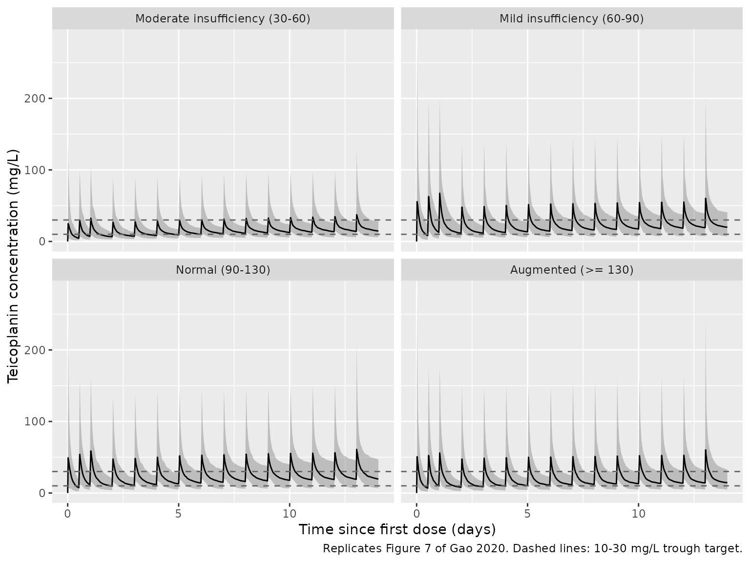
Figure 7 of Gao 2020 shows simulated concentration-time profiles for the recommended regimen in each renal-function group against the 10-30 mg/L trough target. The figure below replicates it with the packaged model (median and 90% prediction interval of 200 virtual children per group).
sim |>
  dplyr::group_by(group, time) |>
  dplyr::summarise(
    Q05 = quantile(Cc, 0.05),
    Q50 = median(Cc),
    Q95 = quantile(Cc, 0.95),
    .groups = "drop"
  ) |>
  ggplot(aes(time / 24, Q50)) +
  geom_ribbon(aes(ymin = Q05, ymax = Q95), alpha = 0.25) +
  geom_line() +
  geom_hline(yintercept = c(10, 30), linetype = "dashed", colour = "grey40") +
  facet_wrap(~group) +
  labs(
    x = "Time since first dose (days)",
    y = "Teicoplanin concentration (mg/L)",
    caption = "Replicates Figure 7 of Gao 2020. Dashed lines: 10-30 mg/L trough target."
  )
PKNCA validation
Steady state is approached slowly (terminal half-life of several days), so NCA is computed over the last simulated dosing interval (312-336 h, day 14). Gao 2020 does not tabulate NCA parameters; the relevant published targets are the 10-30 mg/L trough window and a peak kept at or below about 80 mg/L (Discussion).
ss_start <- 312
ss_end <- 336

conc_df <- sim |>
  dplyr::filter(!is.na(Cc), time >= ss_start, time <= ss_end) |>
  dplyr::select(id, time, Cc, group)

dose_df <- events |>
  dplyr::filter(evid == 1, time >= ss_start, time < ss_end) |>
  dplyr::select(id, time, amt, group)

conc_obj <- PKNCA::PKNCAconc(conc_df, Cc ~ time | group + id, concu = "mg/L", timeu = "h")
dose_obj <- PKNCA::PKNCAdose(dose_df, amt ~ time | group + id, doseu = "mg")
intervals <- data.frame(
  start = ss_start, end = ss_end,
  cmax = TRUE, tmax = TRUE, cmin = TRUE, auclast = TRUE, cav = TRUE
)
nca_res <- PKNCA::pk.nca(PKNCA::PKNCAdata(conc_obj, dose_obj, intervals = intervals))
knitr::kable(
  summary(nca_res),
  caption = "Simulated NCA over the day-14 dosing interval by renal-function group."
)| Interval Start | Interval End | group | N | AUClast (h*mg/L) | Cmax (mg/L) | Cmin (mg/L) | Tmax (h) | Cav (mg/L) |
|---|---|---|---|---|---|---|---|---|
| 312 | 336 | Moderate insufficiency (30-60) | 200 | 479 [41.5] | 40.7 [79.0] | 14.0 [48.7] | 0.500 [0.500, 0.500] | 20.0 [41.5] |
| 312 | 336 | Mild insufficiency (60-90) | 200 | 677 [40.1] | 63.4 [82.5] | 18.8 [52.8] | 0.500 [0.500, 0.500] | 28.2 [40.1] |
| 312 | 336 | Normal (90-130) | 200 | 696 [41.1] | 65.2 [73.2] | 18.4 [56.2] | 0.500 [0.500, 0.500] | 29.0 [41.1] |
| 312 | 336 | Augmented (>= 130) | 200 | 578 [44.1] | 63.2 [92.7] | 13.8 [68.5] | 0.500 [0.500, 0.500] | 24.1 [44.1] |
Comparison against the published dosing targets
trough <- sim |>
  dplyr::filter(time == ss_end) |>
  dplyr::group_by(group) |>
  dplyr::summarise(
    median_trough = median(Cc),
    pct_in_target = 100 * mean(Cc >= 10 & Cc <= 30),
    .groups = "drop"
  )
peak <- sim |>
  dplyr::filter(time > ss_start, time <= ss_start + 2) |>
  dplyr::group_by(group, id) |>
  dplyr::summarise(cmax = max(Cc), .groups = "drop") |>
  dplyr::group_by(group) |>
  dplyr::summarise(median_peak = median(cmax), .groups = "drop")

tgt <- dplyr::left_join(trough, peak, by = "group")
knitr::kable(
  tgt |>
    dplyr::mutate(dplyr::across(where(is.numeric), \(x) round(x, 1))) |>
    dplyr::rename(
      "Renal group" = group,
      "Median trough, day 14 (mg/L)" = median_trough,
      "Trough in 10-30 mg/L (%)" = pct_in_target,
      "Median peak, day 14 (mg/L)" = median_peak
    ),
  caption = "Trough and peak under the regimens Gao 2020 recommends for each renal-function group."
)| Renal group | Median trough, day 14 (mg/L) | Trough in 10-30 mg/L (%) | Median peak, day 14 (mg/L) |
|---|---|---|---|
| Moderate insufficiency (30-60) | 14.5 | 74.0 | 37.4 |
| Mild insufficiency (60-90) | 19.8 | 70.0 | 60.2 |
| Normal (90-130) | 19.5 | 72.0 | 61.0 |
| Augmented (>= 130) | 14.5 | 66.5 | 60.3 |
Assumptions and deviations
-
IIV scale. Table 4 lists omega in percent and its
footnote defines it as the “square root of inter-individual variance”.
The variances in
ini()are therefore (omega/100)^2 (e.g. V1: 1.0543^2 = 1.1116), not log(CV^2 + 1). -
Residual error. Eq. 5 is
Y = IPRED + IPRED^power * epswith the power reported as 0.5 in the Results text. The power does not appear in Table 4, so it is treated as fixed at 0.5 (powExp <- fixed(0.5)), and sigma = 0.46 is taken to be the standard deviation of eps (Cc ~ pow(propSd, powExp)). - V1 weight term. Eq. 15 divides ln(WT) by the printed constant 2.3 (approximately ln(10), the log of the median weight); the printed value is used as-is. The term is undefined for WT <= 1 kg, which is below the study’s weight range (3.5-38 kg).
-
eGFR column. The modified (bedside) Schwartz eGFR
is stored in the canonical
CRCLcolumn in mL/min/1.73 m^2. - Infusion duration. The paper states only “intravenous infusion”; the simulations use a 30-minute infusion.
- Virtual cohort. Weight is drawn log-normal around 10 kg (SD 0.5 on the log scale) truncated to 3.5-38 kg; eGFR is uniform within each group’s band (augmented capped at 200 mL/min/1.73 m^2). The paper does not describe the covariate distributions used for Figure 7.
- Age. Age-based maturation and age-dependent allometric exponents were tested (Table 2, Models II and IV) but the final model uses the simple weight power model; age is not a covariate. The model was developed in children aged 2 months to 9.4 years and should not be extrapolated to neonates.