Piperacillin (Thorsted 2019)

Model and source

• Citation: Thorsted A, Kristoffersson AN, Maarbjerg SF, Schroder H, Wang M, Brock B, Nielsen EI, Friberg LE. (2019). Population pharmacokinetics of piperacillin in febrile children receiving cancer chemotherapy: the impact of body weight and target on an optimal dosing regimen. J Antimicrob Chemother 74(10):2984-2993. doi:10.1093/jac/dkz270. Erratum: J Antimicrob Chemother 2020;75(1):254-255, doi:10.1093/jac/dkz429 (corrects a Results sentence and Figure 5 only; no model parameter changed).
• Description: Two-compartment IV population PK model for UNBOUND (free, ultrafiltrate) piperacillin in febrile children aged 1-18 years receiving cancer chemotherapy (Thorsted 2019). Body weight enters every clearance and volume through fixed-exponent allometry (0.75 on CL and Q, 1.0 on Vc and Vp) referenced to 70 kg. Unexplained variability in clearance is carried entirely as inter-occasion variability between febrile episodes (up to four episodes per child); inter-individual variability became insignificant once the between-episode term was added and is not part of the final model. Proportional residual error.
• Article: https://doi.org/10.1093/jac/dkz270 (open access, PMC6916132)

Population

Thorsted et al. 2019 studied 43 children (aged 1-18 years, median 12) with cancer and chemotherapy-induced fever at the Department of Pediatric Oncology, Aarhus University Hospital, Denmark (April 2016 - January 2018). Children could contribute more than one febrile episode, and 89 episodes (1-4 per child) were analysed. Piperacillin/tazobactam (8:1) was given as a 5-minute IV infusion approximately every 8 h at 300 mg/kg/day piperacillin, capped at the adult 16000 mg/day. The 482 serum samples (19 below the 0.5 mg/L LLOQ, handled with the M3 method) were assayed for unbound piperacillin by UPLC after ultrafiltration, so the model describes free concentrations directly. Episode-level body weight had median 39.4 kg (range 9.5-107) and the Schwartz-estimated GFR a median of 172.4 mL/min/1.73 m^2, i.e. a hyperfiltrating population; 63% of the children were male, neutropenia was present in 87% of episodes and bacteraemia in 11% (Table 1).

Source trace

Model element	Value	Source location
Two-compartment disposition, first-order elimination from central	–	Results, ‘Pharmacokinetic modelling’ (dOFV = -18.7 vs one-compartment)
lcl	log(15.4 L/h) at 70 kg	Table 2
lvc	log(16.0 L) at 70 kg	Table 2
lq	log(0.237 L/h) at 70 kg	Table 2
lvp	log(3.40 L) at 70 kg	Table 2
e_wt_cl, e_wt_q	fixed 0.75	Methods ‘Pharmacokinetic modelling’; Table 2 footnote b
e_wt_vc, e_wt_vp	fixed 1.0	Methods ‘Pharmacokinetic modelling’; Table 2 footnote b
Allometric reference weight	70 kg	Table 2 footnote b
etaiov_cl_1 … etaiov_cl_4	log(1 + 0.166^2) = 0.027183	Table 2 ‘CV%CL’ 16.6%, inter-fever-episode variability
No IIV on any parameter	–	Results: IIV ‘became insignificant’ once IOV was added
propSd	0.332	Table 2 ‘CV%ERR’ 33.2%
Occasion = febrile episode, 1-4 per child	–	Methods ‘Pharmacokinetic modelling’; Results ‘Patient characteristics’

Model

mod <- readModelDb("Thorsted_2019_piperacillin")
mod_typical <- rxode2::zeroRe(mod)
#> Warning: some etas defaulted to non-mu referenced, possible parsing error: etaiov_cl_1, etaiov_cl_2, etaiov_cl_3, etaiov_cl_4
#> as a work-around try putting the mu-referenced expression on a simple line
#> Warning: some etas defaulted to non-mu referenced, possible parsing error: etaiov_cl_1, etaiov_cl_2, etaiov_cl_3, etaiov_cl_4
#> as a work-around try putting the mu-referenced expression on a simple line

Closed-form half-lives

The paper reports distribution and terminal half-lives of 0.708 h and 10.1 h for a 70-kg patient. These follow exactly from the Table 2 parameters through the two-compartment eigenvalues, so this is a tight transcription gate.

cl <- 15.4
vc <- 16.0
q <- 0.237
vp <- 3.40
k10 <- cl / vc
k12 <- q / vc
k21 <- q / vp
s <- k10 + k12 + k21
alpha <- (s + sqrt(s^2 - 4 * k10 * k21)) / 2
beta <- (s - sqrt(s^2 - 4 * k10 * k21)) / 2
hl <- c(alpha = log(2) / alpha, beta = log(2) / beta)
knitr::kable(
  data.frame(
    "Half-life" = c("t1/2,alpha (h)", "t1/2,beta (h)"),
    Paper = c(0.708, 10.1),
    Model = signif(hl, 3),
    check.names = FALSE
  )
)

	Half-life	Paper	Model
alpha	t1/2,alpha (h)	0.708	0.708
beta	t1/2,beta (h)	10.100	10.100

stopifnot(abs(hl[["alpha"]] - 0.708) < 0.005, abs(hl[["beta"]] - 10.1) < 0.05)

Typical concentration-time courses (Figure 3)

Figure 3 shows typical free concentrations for 15, 40 and 65 kg children given 300 mg/kg/day (capped at 16000 mg/day) as (a) three 5-minute infusions, (b) three 3-hour infusions, and (c) a continuous infusion.

wts <- c(15, 40, 65)
daily_dose <- function(wt) min(300 * wt, 16000)

make_regimen <- function(wt, regimen) {
  dd <- daily_dose(wt)
  ev <- switch(regimen,
    "SI 5 min q8h" = rxode2::et(amt = dd / 3, dur = 5 / 60, ii = 8, addl = 2, cmt = "central"),
    "EI 3 h q8h" = rxode2::et(amt = dd / 3, dur = 3, ii = 8, addl = 2, cmt = "central"),
    "CI" = rxode2::et(amt = dd, dur = 24, cmt = "central")
  )
  ev <- rxode2::et(ev, seq(0, 24, by = 0.05), cmt = "central")
  d <- as.data.frame(ev)
  d$WT <- wt
  d$OCC <- 1
  d$id <- 1
  d
}

grid <- expand.grid(wt = wts, regimen = c("SI 5 min q8h", "EI 3 h q8h", "CI"), stringsAsFactors = FALSE)
fig3 <- Map(function(wt, regimen) {
  s <- rxode2::rxSolve(mod_typical, make_regimen(wt, regimen), returnType = "data.frame")
  data.frame(time = s$time, Cc = s$Cc, wt = paste(wt, "kg"), regimen = regimen)
}, grid$wt, grid$regimen) |>
  dplyr::bind_rows() |>
  dplyr::mutate(regimen = factor(regimen, levels = c("SI 5 min q8h", "EI 3 h q8h", "CI")))
#> ℹ omega/sigma items treated as zero: 'etaiov_cl_1', 'etaiov_cl_2', 'etaiov_cl_3', 'etaiov_cl_4'
#> ℹ omega/sigma items treated as zero: 'etaiov_cl_1', 'etaiov_cl_2', 'etaiov_cl_3', 'etaiov_cl_4'
#> ℹ omega/sigma items treated as zero: 'etaiov_cl_1', 'etaiov_cl_2', 'etaiov_cl_3', 'etaiov_cl_4'
#> ℹ omega/sigma items treated as zero: 'etaiov_cl_1', 'etaiov_cl_2', 'etaiov_cl_3', 'etaiov_cl_4'
#> ℹ omega/sigma items treated as zero: 'etaiov_cl_1', 'etaiov_cl_2', 'etaiov_cl_3', 'etaiov_cl_4'
#> ℹ omega/sigma items treated as zero: 'etaiov_cl_1', 'etaiov_cl_2', 'etaiov_cl_3', 'etaiov_cl_4'
#> ℹ omega/sigma items treated as zero: 'etaiov_cl_1', 'etaiov_cl_2', 'etaiov_cl_3', 'etaiov_cl_4'
#> ℹ omega/sigma items treated as zero: 'etaiov_cl_1', 'etaiov_cl_2', 'etaiov_cl_3', 'etaiov_cl_4'
#> ℹ omega/sigma items treated as zero: 'etaiov_cl_1', 'etaiov_cl_2', 'etaiov_cl_3', 'etaiov_cl_4'

ggplot(fig3, aes(time, Cc, colour = wt)) +
  geom_line() +
  geom_hline(yintercept = c(0.5, 2, 4, 16), linetype = "dashed", colour = "grey50") +
  facet_wrap(~regimen) +
  scale_y_log10() +
  scale_x_continuous(breaks = seq(0, 24, 8)) +
  labs(
    x = "Time (h)", y = "Unbound piperacillin (mg/L)", colour = "Body weight",
    caption = "Replicates Figure 3 of Thorsted 2019 (typical patient, 300 mg/kg/day)."
  )
#> Warning in scale_y_log10(): log-10 transformation introduced infinite values.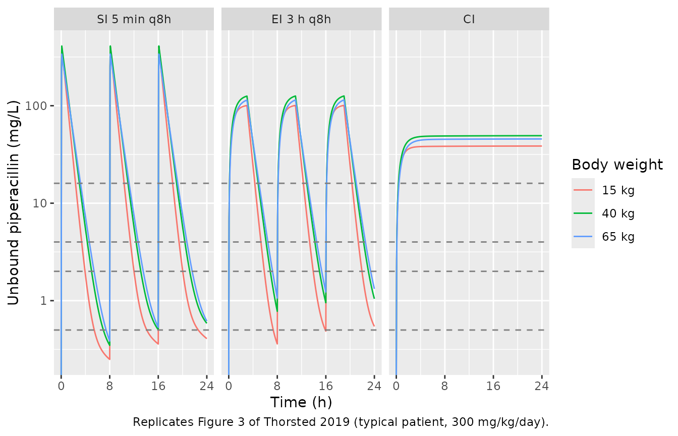

Consistent with the paper, lighter children reach lower troughs because the allometric exponent on CL (0.75) is smaller than on volume (1.0), which shortens their half-life. After the 5-minute infusion the peaks sit in the few hundred mg/L range (about 340-410 mg/L in the first interval; the paper quotes roughly 500 mg/L, read by eye from its log-scale Figure 3).

peaks <- fig3 |>
  dplyr::filter(regimen == "SI 5 min q8h", time <= 8) |>
  dplyr::group_by(wt) |>
  dplyr::summarise(Cmax = max(Cc), C8 = Cc[which.min(abs(time - 8))], .groups = "drop")
knitr::kable(peaks, digits = 2)

wt	Cmax	C8
15 kg	402.58	0.25
40 kg	409.88	0.35
65 kg	338.82	0.39

# Peaks after the 5-min infusion stay at or below the paper's ~500 mg/L.
stopifnot(all(peaks$Cmax < 550), all(peaks$Cmax > 250))

Dose required for target attainment (Figure 5)

The corrected Figure 5 (erratum doi:10.1093/jac/dkz429) prints, for typical 15, 40 and 65 kg children at MIC = 4 mg/L (the MIC90), the steady-state dose required for each target together with the resulting AUCss and Cmax,ss, for (a) the licensed regimen (30-minute infusion q6h) and (b) a 3-hour extended infusion q8h.

fig5_ref <- data.frame(
  regimen = rep(c("(a) 30 min q6h", "(b) EI 3 h q8h"), each = 6),
  target = rep(rep(c("50% fT>4xMIC", "100% fT>MIC"), each = 3), 2),
  wt = rep(c(15, 40, 65), 4),
  dose_mg = c(2353, 2803, 3459, 7078, 9254, 10299, 1203, 1984, 2652, 10095, 13800, 14625),
  auclast = c(518.5, 296.1, 237.9, 1560, 977.3, 708.4, 248.5, 196.6, 182.4, 2087, 1365, 1007),
  cmax = c(526.9, 251.4, 185.2, 1585, 829.7, 551.3, 81.1, 63.3, 57.3, 680.4, 439.2, 316.4)
)
fig5_ref$treatment <- paste(fig5_ref$regimen, fig5_ref$target, paste(fig5_ref$wt, "kg"), sep = " | ")

Because the model is linear, the steady-state profile scales with dose, so the required dose is found by bisection on one steady-state profile per weight and regimen. The threshold is 16 mg/L for 50% fT>4xMIC and 4 mg/L for 100% fT>MIC.

ss_profile <- function(wt, tau, tinf, amt = 100 * wt, n = 40, by = 0.005) {
  ev <- rxode2::et(amt = amt, dur = tinf, ii = tau, addl = n - 1, cmt = "central")
  ev <- rxode2::et(ev, seq((n - 1) * tau, n * tau, by = by), cmt = "central")
  d <- as.data.frame(ev)
  d$WT <- wt
  d$OCC <- 1
  d$id <- 1
  s <- rxode2::rxSolve(mod_typical, d, returnType = "data.frame")
  s <- s[s$time >= (n - 1) * tau, ]
  data.frame(time = s$time - (n - 1) * tau, Cc = s$Cc, c_per_mg = s$Cc / amt)
}

required_dose <- function(p, threshold, frac) {
  ft <- function(dose) mean(p$c_per_mg * dose > threshold)
  lo <- 1
  hi <- 1e6
  for (i in 1:60) {
    mid <- sqrt(lo * hi)
    if (ft(mid) >= frac) hi <- mid else lo <- mid
  }
  hi
}

regimens <- list(
  "(a) 30 min q6h" = c(tau = 6, tinf = 0.5),
  "(b) EI 3 h q8h" = c(tau = 8, tinf = 3)
)
thresholds <- list("50% fT>4xMIC" = c(thr = 16, frac = 0.5), "100% fT>MIC" = c(thr = 4, frac = 1))

fig5_sim <- fig5_ref[, c("regimen", "target", "wt", "treatment")]
fig5_sim$dose_mg <- NA_real_
for (i in seq_len(nrow(fig5_sim))) {
  r <- regimens[[fig5_sim$regimen[i]]]
  th <- thresholds[[fig5_sim$target[i]]]
  p <- ss_profile(fig5_sim$wt[i], r[["tau"]], r[["tinf"]])
  fig5_sim$dose_mg[i] <- required_dose(p, th[["thr"]], th[["frac"]])
}
#> ℹ omega/sigma items treated as zero: 'etaiov_cl_1', 'etaiov_cl_2', 'etaiov_cl_3', 'etaiov_cl_4'
#> ℹ omega/sigma items treated as zero: 'etaiov_cl_1', 'etaiov_cl_2', 'etaiov_cl_3', 'etaiov_cl_4'
#> ℹ omega/sigma items treated as zero: 'etaiov_cl_1', 'etaiov_cl_2', 'etaiov_cl_3', 'etaiov_cl_4'
#> ℹ omega/sigma items treated as zero: 'etaiov_cl_1', 'etaiov_cl_2', 'etaiov_cl_3', 'etaiov_cl_4'
#> ℹ omega/sigma items treated as zero: 'etaiov_cl_1', 'etaiov_cl_2', 'etaiov_cl_3', 'etaiov_cl_4'
#> ℹ omega/sigma items treated as zero: 'etaiov_cl_1', 'etaiov_cl_2', 'etaiov_cl_3', 'etaiov_cl_4'
#> ℹ omega/sigma items treated as zero: 'etaiov_cl_1', 'etaiov_cl_2', 'etaiov_cl_3', 'etaiov_cl_4'
#> ℹ omega/sigma items treated as zero: 'etaiov_cl_1', 'etaiov_cl_2', 'etaiov_cl_3', 'etaiov_cl_4'
#> ℹ omega/sigma items treated as zero: 'etaiov_cl_1', 'etaiov_cl_2', 'etaiov_cl_3', 'etaiov_cl_4'
#> ℹ omega/sigma items treated as zero: 'etaiov_cl_1', 'etaiov_cl_2', 'etaiov_cl_3', 'etaiov_cl_4'
#> ℹ omega/sigma items treated as zero: 'etaiov_cl_1', 'etaiov_cl_2', 'etaiov_cl_3', 'etaiov_cl_4'
#> ℹ omega/sigma items treated as zero: 'etaiov_cl_1', 'etaiov_cl_2', 'etaiov_cl_3', 'etaiov_cl_4'

dose_cmp <- merge(
  fig5_ref[, c("treatment", "dose_mg")], fig5_sim[, c("treatment", "dose_mg")],
  by = "treatment", suffixes = c("_paper", "_model")
)
dose_cmp$pct_diff <- 100 * (dose_cmp$dose_mg_model / dose_cmp$dose_mg_paper - 1)
dose_cmp |>
  dplyr::rename(
    "Regimen | target | weight" = treatment,
    "Paper dose (mg)" = dose_mg_paper,
    "Model dose (mg)" = dose_mg_model,
    "% diff" = pct_diff
  ) |>
  knitr::kable(digits = 1)

Regimen | target | weight	Paper dose (mg)	Model dose (mg)	% diff
(a) 30 min q6h | 100% fT>MIC | 15 kg	7078	7604.8	7.4
(a) 30 min q6h | 100% fT>MIC | 40 kg	9254	9956.7	7.6
(a) 30 min q6h | 100% fT>MIC | 65 kg	10299	10386.4	0.8
(a) 30 min q6h | 50% fT>4xMIC | 15 kg	2353	2568.0	9.1
(a) 30 min q6h | 50% fT>4xMIC | 40 kg	2803	3094.7	10.4
(a) 30 min q6h | 50% fT>4xMIC | 65 kg	3459	3600.6	4.1
(b) EI 3 h q8h | 100% fT>MIC | 15 kg	10095	10170.2	0.7
(b) EI 3 h q8h | 100% fT>MIC | 40 kg	13800	13901.4	0.7
(b) EI 3 h q8h | 100% fT>MIC | 65 kg	14625	14750.4	0.9
(b) EI 3 h q8h | 50% fT>4xMIC | 15 kg	1203	1207.5	0.4
(b) EI 3 h q8h | 50% fT>4xMIC | 40 kg	1984	2016.5	1.6
(b) EI 3 h q8h | 50% fT>4xMIC | 65 kg	2652	2663.5	0.4

For the extended-infusion regimen (panel b) every model dose is within 2% of the published dose, and the two licensed-regimen doses at 65 kg are within 1% and 4%. At 15 and 40 kg the licensed-regimen doses (panel a) come out 7-10% higher than published. This is not a transcription error in the model: panel a is not internally consistent with panel b under any single set of linear PK parameters. The steady-state AUC over a dosing interval equals dose / CL whatever the regimen, so the paper’s own dose / AUCss ratio recovers the clearance it simulated with:

fig5_ref |>
  dplyr::filter(target == "50% fT>4xMIC") |>
  dplyr::mutate(cl_implied = dose_mg / auclast, cl_model = 15.4 * (wt / 70)^0.75) |>
  dplyr::select(regimen, wt, cl_implied, cl_model) |>
  dplyr::rename(
    "Regimen" = regimen, "Body weight (kg)" = wt,
    "Paper dose / AUCss (L/h)" = cl_implied, "Model CL (L/h)" = cl_model
  ) |>
  knitr::kable(digits = 2)

Regimen	Body weight (kg)	Paper dose / AUCss (L/h)	Model CL (L/h)
(a) 30 min q6h	15	4.54	4.85
(a) 30 min q6h	40	9.47	10.12
(a) 30 min q6h	65	14.54	14.57
(b) EI 3 h q8h	15	4.84	4.85
(b) EI 3 h q8h	40	10.09	10.12
(b) EI 3 h q8h	65	14.54	14.57

Panel b implies the Table 2 clearance at every weight, and so does panel a at 65 kg, but at 15 and 40 kg panel a implies a clearance about 6% lower – the same size as the dose gap. The erratum already corrected dose and AUC values in this figure once; the residual inconsistency is recorded here and not tuned away. The Results text quotes panel a as 0.67-1.96 (50% fT>4xMIC) and 1.98-5.78 (100% fT>MIC) times 80 mg/kg.

b <- dose_cmp$pct_diff[grepl("^\\(b\\)", dose_cmp$treatment)]
a65 <- dose_cmp$pct_diff[grepl("^\\(a\\).*65 kg$", dose_cmp$treatment)]
a_all <- dose_cmp$pct_diff[grepl("^\\(a\\)", dose_cmp$treatment)]
# Deterministic typical-value calculations: tight where the paper is
# self-consistent, a documented envelope for the self-inconsistent panel a.
stopifnot(all(abs(b) < 3), all(abs(a65) < 5), all(abs(a_all) < 12))

Steady-state exposure with PKNCA (Figure 5)

The typical steady-state interval at each model-derived dose is analysed with PKNCA (one typical profile per regimen, target and weight) and compared with the AUCss and Cmax,ss printed in Figure 5.

conc <- lapply(seq_len(nrow(fig5_sim)), function(i) {
  r <- regimens[[fig5_sim$regimen[i]]]
  p <- ss_profile(fig5_sim$wt[i], r[["tau"]], r[["tinf"]], amt = fig5_sim$dose_mg[i], by = 0.02)
  data.frame(id = i, treatment = fig5_sim$treatment[i], time = p$time, Cc = p$Cc)
}) |>
  dplyr::bind_rows() |>
  dplyr::filter(!is.na(Cc))
#> ℹ omega/sigma items treated as zero: 'etaiov_cl_1', 'etaiov_cl_2', 'etaiov_cl_3', 'etaiov_cl_4'
#> ℹ omega/sigma items treated as zero: 'etaiov_cl_1', 'etaiov_cl_2', 'etaiov_cl_3', 'etaiov_cl_4'
#> ℹ omega/sigma items treated as zero: 'etaiov_cl_1', 'etaiov_cl_2', 'etaiov_cl_3', 'etaiov_cl_4'
#> ℹ omega/sigma items treated as zero: 'etaiov_cl_1', 'etaiov_cl_2', 'etaiov_cl_3', 'etaiov_cl_4'
#> ℹ omega/sigma items treated as zero: 'etaiov_cl_1', 'etaiov_cl_2', 'etaiov_cl_3', 'etaiov_cl_4'
#> ℹ omega/sigma items treated as zero: 'etaiov_cl_1', 'etaiov_cl_2', 'etaiov_cl_3', 'etaiov_cl_4'
#> ℹ omega/sigma items treated as zero: 'etaiov_cl_1', 'etaiov_cl_2', 'etaiov_cl_3', 'etaiov_cl_4'
#> ℹ omega/sigma items treated as zero: 'etaiov_cl_1', 'etaiov_cl_2', 'etaiov_cl_3', 'etaiov_cl_4'
#> ℹ omega/sigma items treated as zero: 'etaiov_cl_1', 'etaiov_cl_2', 'etaiov_cl_3', 'etaiov_cl_4'
#> ℹ omega/sigma items treated as zero: 'etaiov_cl_1', 'etaiov_cl_2', 'etaiov_cl_3', 'etaiov_cl_4'
#> ℹ omega/sigma items treated as zero: 'etaiov_cl_1', 'etaiov_cl_2', 'etaiov_cl_3', 'etaiov_cl_4'
#> ℹ omega/sigma items treated as zero: 'etaiov_cl_1', 'etaiov_cl_2', 'etaiov_cl_3', 'etaiov_cl_4'
doses <- data.frame(id = seq_len(nrow(fig5_sim)), treatment = fig5_sim$treatment, time = 0, amt = fig5_sim$dose_mg)
tau_by_id <- ifelse(grepl("^\\(a\\)", fig5_sim$treatment), 6, 8)
intervals <- data.frame(
  id = seq_len(nrow(fig5_sim)), treatment = fig5_sim$treatment,
  start = 0, end = tau_by_id, auclast = TRUE, cmax = TRUE
)

conc_obj <- PKNCA::PKNCAconc(conc, Cc ~ time | treatment + id)
dose_obj <- PKNCA::PKNCAdose(doses, amt ~ time | treatment + id)
nca <- PKNCA::pk.nca(PKNCA::PKNCAdata(conc_obj, dose_obj, intervals = intervals))

tbl <- nlmixr2lib::ncaComparisonTable(
  nca, fig5_ref[, c("treatment", "auclast", "cmax")],
  by = "treatment",
  units = c(auclast = "mg*h/L", cmax = "mg/L")
)
knitr::kable(tbl)

NCA parameter	treatment	Reference	Simulated	% diff
Cmax (mg/L)	(a) 30 min q6h | 50% fT>4xMIC | 15 kg	527	536	+1.6%
Cmax (mg/L)	(a) 30 min q6h | 50% fT>4xMIC | 40 kg	251	260	+3.4%
Cmax (mg/L)	(a) 30 min q6h | 50% fT>4xMIC | 65 kg	185	192	+3.7%
Cmax (mg/L)	(a) 30 min q6h | 100% fT>MIC | 15 kg	1580	1590	+0.1%
Cmax (mg/L)	(a) 30 min q6h | 100% fT>MIC | 40 kg	830	836	+0.8%
Cmax (mg/L)	(a) 30 min q6h | 100% fT>MIC | 65 kg	551	554	+0.4%
Cmax (mg/L)	(b) EI 3 h q8h | 50% fT>4xMIC | 15 kg	81.1	81.1	+0.0%
Cmax (mg/L)	(b) EI 3 h q8h | 50% fT>4xMIC | 40 kg	63.3	63.5	+0.4%
Cmax (mg/L)	(b) EI 3 h q8h | 50% fT>4xMIC | 65 kg	57.3	57.4	+0.1%
Cmax (mg/L)	(b) EI 3 h q8h | 100% fT>MIC | 15 kg	680	683	+0.4%
Cmax (mg/L)	(b) EI 3 h q8h | 100% fT>MIC | 40 kg	439	438	-0.3%
Cmax (mg/L)	(b) EI 3 h q8h | 100% fT>MIC | 65 kg	316	318	+0.4%
AUClast (mg*h/L)	(a) 30 min q6h | 50% fT>4xMIC | 15 kg	518	529	+2.1%
AUClast (mg*h/L)	(a) 30 min q6h | 50% fT>4xMIC | 40 kg	296	306	+3.3%
AUClast (mg*h/L)	(a) 30 min q6h | 50% fT>4xMIC | 65 kg	238	247	+3.9%
AUClast (mg*h/L)	(a) 30 min q6h | 100% fT>MIC | 15 kg	1560	1570	+0.5%
AUClast (mg*h/L)	(a) 30 min q6h | 100% fT>MIC | 40 kg	977	984	+0.7%
AUClast (mg*h/L)	(a) 30 min q6h | 100% fT>MIC | 65 kg	708	713	+0.6%
AUClast (mg*h/L)	(b) EI 3 h q8h | 50% fT>4xMIC | 15 kg	248	249	+0.2%
AUClast (mg*h/L)	(b) EI 3 h q8h | 50% fT>4xMIC | 40 kg	197	199	+1.3%
AUClast (mg*h/L)	(b) EI 3 h q8h | 50% fT>4xMIC | 65 kg	182	183	+0.2%
AUClast (mg*h/L)	(b) EI 3 h q8h | 100% fT>MIC | 15 kg	2090	2100	+0.5%
AUClast (mg*h/L)	(b) EI 3 h q8h | 100% fT>MIC | 40 kg	1360	1370	+0.6%
AUClast (mg*h/L)	(b) EI 3 h q8h | 100% fT>MIC | 65 kg	1010	1010	+0.6%

Starred rows (> 20% difference) would flag a problem; the AUC and Cmax rows follow the dose comparison above (panel b and 65 kg within a few percent, the self-inconsistent panel a rows at 15 and 40 kg somewhat further off).

res <- as.data.frame(nca$result)
chk <- merge(
  res[res$PPTESTCD %in% c("auclast", "cmax"), c("treatment", "PPTESTCD", "PPORRES")],
  tidyr::pivot_longer(fig5_ref[, c("treatment", "auclast", "cmax")], -treatment,
    names_to = "PPTESTCD", values_to = "ref"
  ),
  by = c("treatment", "PPTESTCD")
)
chk$pct <- 100 * (chk$PPORRES / chk$ref - 1)
stopifnot(
  all(abs(chk$pct[grepl("^\\(b\\)", chk$treatment)]) < 5),
  all(abs(chk$pct) < 20)
)

Variability around the typical profile (Figure 5b)

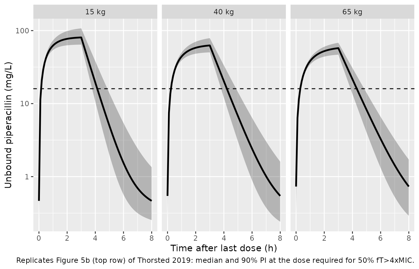
A stochastic cohort of 200 episodes per weight (IOV on CL, one episode each, proportional residual error excluded as in a prediction interval of the typical profile) reproduces the 90% prediction interval of the 50% fT>4xMIC extended-infusion panel of Figure 5b.

rxode2::rxSetSeed(20190827)
n_per_arm <- 200
n_dose <- 10
tau <- 8
ei50 <- fig5_sim[fig5_sim$regimen == "(b) EI 3 h q8h" & fig5_sim$target == "50% fT>4xMIC", ]
cohort <- lapply(seq_len(nrow(ei50)), function(i) {
  ev <- rxode2::et(amt = ei50$dose_mg[i], dur = 3, ii = tau, addl = n_dose - 1, cmt = "central")
  ev <- rxode2::et(ev, seq((n_dose - 1) * tau, n_dose * tau, by = 0.1), cmt = "central")
  d <- as.data.frame(ev)
  ids <- seq_len(n_per_arm) + (i - 1) * n_per_arm
  d <- dplyr::bind_rows(lapply(ids, function(id) dplyr::mutate(d, id = id)))
  d$WT <- ei50$wt[i]
  d$OCC <- 1
  d$weight <- paste(ei50$wt[i], "kg")
  d
}) |> dplyr::bind_rows()

sim <- rxode2::rxSolve(mod, cohort, keep = "weight", returnType = "data.frame")
#> Warning: some etas defaulted to non-mu referenced, possible parsing error: etaiov_cl_1, etaiov_cl_2, etaiov_cl_3, etaiov_cl_4
#> as a work-around try putting the mu-referenced expression on a simple line
pi_df <- sim |>
  dplyr::filter(time >= (n_dose - 1) * tau) |>
  dplyr::mutate(tad = time - (n_dose - 1) * tau) |>
  dplyr::group_by(weight, tad) |>
  dplyr::summarise(med = median(Cc), lo = quantile(Cc, 0.05), hi = quantile(Cc, 0.95), .groups = "drop")

ggplot(pi_df, aes(tad, med)) +
  geom_ribbon(aes(ymin = lo, ymax = hi), alpha = 0.3) +
  geom_line(linewidth = 1) +
  geom_hline(yintercept = 16, linetype = "dashed") +
  facet_wrap(~weight) +
  scale_y_log10() +
  labs(
    x = "Time after last dose (h)", y = "Unbound piperacillin (mg/L)",
    caption = "Replicates Figure 5b (top row) of Thorsted 2019: median and 90% PI at the dose required for 50% fT>4xMIC."
  )

Assumptions and deviations

• IOV encoding. The paper’s only random effect on a structural parameter is inter-occasion (between-febrile-episode) variability on CL, with no IIV in the final model. rxode2 cannot simulate the eta ~ var | occ syntax, so the model multiplexes four per-occasion etas through the canonical OCC column (children contributed 1-4 episodes), with occasions 2-4 fixed to the occasion-1 variance. Because there is no IIV, simulating each episode as a separate subject with OCC = 1 (as done above) is statistically equivalent.
• CV to variance. Table 2 reports the IOV as 16.6% CV; it was converted to a log-scale variance with log(1 + CV^2). The proportional residual CV of 33.2% is used directly as propSd.
• Allometric exponent on Q. Table 2 footnote b states the 0.75 exponent for “CL”; the Methods state 0.75 applies to clearances in general, so it is also applied to Q.
• Figure 5a self-inconsistency. At 15 and 40 kg the licensed-regimen panel implies (through dose / AUCss) a clearance about 6% below the Table 2 value that panel b and the 65-kg panel a reproduce, and the model-derived required doses are correspondingly 7-10% higher. The model was not adjusted; the gap is reported in the comparison tables above.
• Target attainment definition. fT>threshold is computed on a 0.005-h grid over one steady-state dosing interval of the typical (no IOV) profile; the paper does not state its grid, which may explain the remaining 1-2% differences in panel b.
• Unbound concentrations. Cc is the free (ultrafiltrate) serum concentration; no protein-binding correction should be applied when using the model for fT>MIC.
• Tazobactam was not measured and is not modelled.
• Erratum (doi:10.1093/jac/dkz429, J Antimicrob Chemother 2020;75:254-255) corrects the Results sentence on the licensed regimen (the 100% fT>MIC range was misprinted as 2.10-9.25 and should read 1.98-5.78 times 80 mg/kg) and some dose / AUCss values in Figure 5. No model parameter or equation is affected. The corrected 1.98-5.78 range is the one checked above. The Discussion’s 182-248 mg*h/L AUC range was not amended by the erratum.
• Appendix S1 (supplementary data) describes the optimal sampling design only and carries no parameters of the final model.