Momelotinib (Rich 2026)
Source:vignettes/articles/Rich_2026_momelotinib.Rmd
Rich_2026_momelotinib.RmdModel and source
- Citation: Rich B, Srinivasan M, Ho YL, Visser SAG, Ferron-Brady G, Vlasakakis G. Population pharmacokinetics and exposure-response analyses of momelotinib, its active metabolite (M21), and total active moiety in myelofibrosis. Clin Pharmacol Ther. 2026;119(3):629-641. doi:10.1002/cpt.70076. Structural and covariate parameter estimates are from Table 1 and its PK-parameter-equations footnote; the residual-error stratification, the absorption-chain topology and the simulated exposure metrics used to validate this implementation are from Supplemental Tables S3, S5 and S6 (supplement file CPT-119-629-s001). The fraction metabolised fm = 0.640 originates in the human mass-balance study Zheng J et al. Drug Metab Dispos. 2018;46:237-247, doi:10.1124/dmd.117.078030, which also reports the M21 relative potency of approximately 0.4 used to form the total active moiety. The nine exposure-response regressions the same paper reports are NOT extracted: Tables S9 and S10 print no intercept for any of the seven logistic models, and neither table nor the main text reports the centering constant of the log2-transformed exposure metric, so the absolute level of every one of those regressions is unidentified from the published record. See the vignette Errata.
- Article: https://doi.org/10.1002/cpt.70076
- Supplement (open access, EuropePMC
PMC12882756, fileCPT-119-629-s001.docx): https://europepmc.org/article/PMC/PMC12882756
Momelotinib is an oral JAK1 / JAK2 / ACVR1 inhibitor approved for myelofibrosis with anemia. Rich 2026 describes the population pharmacokinetics of momelotinib and of M21, its major circulating metabolite, and then uses the combined potency-weighted “total active moiety” (TAM) exposure to explore exposure-response relationships for eight efficacy and safety end points.
This vignette validates the packaged population PK model. The nine exposure-response regressions are not packaged; see Assumptions, deviations and errata for why.
mod <- readModelDb("Rich_2026_momelotinib")
meta <- mod()
Population
The population PK analysis pooled 661 participants across 7 trials (Rich 2026 Supplemental Table S7): 547 patients with intermediate- or high-risk myelofibrosis from the phase II translational-biology study GS-US-352-1672 and the three phase III trials SIMPLIFY-1, SIMPLIFY-2 and MOMENTUM, plus 114 healthy participants or participants with renal or hepatic impairment from the phase I clinical-pharmacology studies GS-US-352-1151 / -1152 / -1153.
Baseline characteristics: age median 66 years (range 18-92), body weight median 74.0 kg (range 34.2-136), 38.6% female, 82.9% White / 5.1% Asian / 3.9% Black. Baseline creatinine clearance (Cockcroft-Gault) median 75.9 mL/min (range 21.6-229). NCI-ODWG hepatic function: 74.7% normal, 19.2% mild, 4.4% moderate, 1.5% severe. The dataset comprised 4508 measurable momelotinib and 4516 measurable M21 plasma concentrations.
All of this is available programmatically from the model’s
population metadata
(readModelDb("Rich_2026_momelotinib")()$population).
Model structure
Momelotinib. A two-compartment disposition model
with first-order elimination, fed by a six-compartment transit
absorption chain. Supplemental Table S3 selected run
mmb-2cmt-erlang6-ka-altv, described as “6 transit comp., 6
ktr transitions followed by ka transition”: the
oral dose lands in depot, six successive ktr
transitions carry it through transit1 …
transit6, and a final, much slower ka step
delivers it to central. Because ka = 0.303 1/h
is far slower than ktr = 8.63 1/h, the
last step is rate-limiting, not the transit chain.
Disposition was parameterised as a total apparent volume
(383 L) with an estimated central fraction (0.289), carrying a single
random effect on the total; the packaged model keeps the canonical
vc / vp names and shares one
etalvc between them, which is algebraically identical.
M21. A two-compartment model with first-order
elimination, formed from eliminated momelotinib in proportion to the
fraction metabolised fm, held at 0.640 from a human
mass-balance study. Rich 2026 fitted M21 sequentially on the
parent’s post hoc predictions; the packaged model couples the two
through fm, which reproduces the published M21 exposure
(checked below). The positive parent-metabolite clearance correlation of
Figure S7 was carried into the sequential M21 fit as a power dependence
of M21 clearance on the individual momelotinib clearance rather than as
an estimated off-diagonal omega.
Total active moiety.
tam = Cc + 0.4 * Cc_m21 (Rich 2026 Simulations).
cat(meta$description)
#> Joint parent + metabolite population pharmacokinetic model for oral momelotinib (a JAK1 / JAK2 / ACVR1 inhibitor approved for myelofibrosis with anemia) and its major active metabolite M21, in 661 participants from four studies in patients with myelofibrosis (the phase II translational-biology study GS-US-352-1672 and the phase III SIMPLIFY-1, SIMPLIFY-2 and MOMENTUM trials) plus three phase I clinical-pharmacology studies in healthy participants and in renal or hepatic impairment (Rich 2026). Momelotinib is described by a two-compartment model with six transit absorption compartments and first-order elimination; the chain is depot -> transit1 ... transit6 at the common transit rate ktr, then a slower first-order ka step into the central compartment. M21 is formed from the eliminated momelotinib in proportion to the fraction metabolised fm (held at 0.640 from a human mass-balance study) and is itself described by a two-compartment model with first-order elimination. Retained momelotinib covariates: NCI-ODWG hepatic impairment and concomitant moderate or strong CYP3A4 inducers on apparent clearance, and concomitant OATP1B1/1B3 inhibitors on relative bioavailability. Retained M21 covariates: a power effect of the individual momelotinib apparent clearance and of baseline creatinine clearance on apparent M21 clearance, and NCI-ODWG hepatic impairment on fm on the logit scale. Residual error is proportional in the phase III studies and proportional-plus-additive in the phase I/II studies, for both analytes. The model also returns the total active moiety tam, the potency-weighted sum of the two concentrations that the companion exposure-response analyses use. The paper fitted momelotinib and M21 SEQUENTIALLY (the M21 run consumed the parent model's post hoc estimates); this file couples them into one rxode2 model through fm, which reproduces the published M21 exposure. See vignette Assumptions and deviations.
Source trace
Every ini() entry in
inst/modeldb/specificDrugs/Rich_2026_momelotinib.R carries
an in-file comment naming its source location. Collected here for
review:
| Equation / parameter | Value | Source location |
|---|---|---|
lcl (CL/F) |
64.7 L/h | Table 1, “CL/F” |
lq (Q/F) |
36.1 L/h | Table 1, “Q/F” |
lvc, lvp
|
0.289 x 383 L, (1 - 0.289) x 383 L | Table 1, “Total V/F” and “Fraction V central”; footnote Vci / Vpi |
lktr |
8.63 1/h | Table 1, “ktr” |
lka |
0.303 1/h | Table 1, “ka” |
lfdepot (Frel reference) |
1 | Table 1 footnote, “Frel,i,j = 1.64 … (otherwise 1)” |
e_hepimp_mild_cl / _mod_ /
_sev_
|
log(0.914), log(0.779), log(0.477) | Table 1, hepatic-dysfunction-on-CL/F rows |
e_cyp3a4_ind_mod_cl |
log(1.39) | Table 1, “Moderate CYP3A4 inducer on CL/F” |
e_cyp3a4_ind_strong_cl |
log(2.01) | Table 1, “Strong CYP3A4 inducer on CL/F” (see Errata) |
e_oatp1b_inh_fdepot |
log(1.64) | Table 1, “OATP1B1/1B3 inhibitor on relative bioavailability” |
etalcl, etalvc, etalktr,
etalka
|
0.650^2, 0.476^2, 0.910^2, 0.532^2 | Table 1, “Interindividual variability” (omega SD scale; see Errata) |
propSdPh3, propSdPh12,
addSdPh12
|
0.584, 0.343, 1.47 ng/mL | Table 1, momelotinib “Residual error” block |
lcl_m21, lvc_m21, lvp_m21,
lq_m21
|
24.9 L/h, 2.77 L, 45.7 L, 8.84 L/h | Table 1, M21 “Typical values” |
logitfm |
logit(0.640) | Methods, “Fmet … fixed at 0.64”; Table 1 footnote |
e_clmmb_cl_m21 |
0.481 | Table 1, “CL/F of momelotinib on CLm/F” |
e_crcl_base_cl_m21 |
0.418 | Table 1, “CrCL at baseline on CLm/F” |
e_hepimp_*_fm |
-0.359, -0.679, -1.84 | Table 1, “… on fraction metabolized (logit scale)” |
etalcl_m21, etalvc_m21
|
0.371^2, 2.39^2 | Table 1, M21 “Interindividual variability” |
propSdPh3_m21, propSdPh12_m21,
addSdPh12_m21
|
0.517, 0.337, 1.86 ng/mL | Table 1 (Continued), M21 “Residual error” |
| Six-transit + ka absorption topology | n/a | Supplemental Table S3, run
mmb-2cmt-erlang6-ka-altv
|
| Phase III vs phase I/II residual split | n/a | Supplemental Table S3, run ...-errph3; Table 1 residual
rows |
tam = Cc + 0.4 * Cc_m21 |
Rp = 0.4 | Simulations; potency from Zheng 2018 (doi:10.1124/dmd.117.078030) |
Reference regimen and covariate helper
All simulations below use the approved 200 mg once-daily regimen dosed to steady state. Doses are given on days 0-19; the interval after the last dose (456-480 h) is the steady-state dosing interval, and 480-600 h is a washout tail used only to estimate the terminal half-life.
dose_amt   <- 200      # mg
tau        <- 24       # h
n_doses    <- 20
last_dose  <- (n_doses - 1) * tau           # 456 h
obs_times  <- c(
  seq(last_dose, last_dose + tau, by = 0.25),
  seq(last_dose + tau + 2, last_dose + 144, by = 2)
)

# Reference covariate vector: normal hepatic function, no interacting
# comedication, median baseline CrCL of the myelofibrosis studies, and the
# phase I/II residual-error stratum (the rich-profile setting).
reference_covariates <- list(
  HEPIMP_MILD              = 0,
  HEPIMP_MOD               = 0,
  HEPIMP_SEV               = 0,
  CONMED_CYP3A4_IND_MOD    = 0,
  CONMED_CYP3A4_IND_STRONG = 0,
  CONMED_OATP1B_INH        = 0,
  CRCL_BASE                = 72,
  STUDY_PHASE3             = 0
)
# Attach a named list of covariate values as columns.
add_covariates <- function(df, covariates) {
  for (nm in names(covariates)) df[[nm]] <- covariates[[nm]]
  df
}

# Build a dosing + observation event table for `n` subjects.
#
# Observation rows carry cmt = "Cc". This model declares TWO endpoints
# (Cc and Cc_m21), and rxode2 requires observation records of a
# multiple-endpoint model to name an endpoint rather than an ODE state --
# observing cmt = "central" errors out. Cc and Cc_m21 already occupy
# compartment slots 12 and 13 by virtue of their residual-error
# declarations, so naming Cc here injects nothing and leaves the eleven
# ODE states in slots 1-11 untouched. rxSolve returns every model
# variable (Cc, Cc_m21, tam) at each observation row regardless.
make_events <- function(n, covariates, scenario = "reference", id_offset = 0L) {
  ids <- id_offset + seq_len(n)
  doses <- tidyr::expand_grid(id = ids, time = seq(0, last_dose, by = tau)) |>
    dplyr::mutate(evid = 1L, amt = dose_amt, cmt = "depot")
  obs <- tidyr::expand_grid(id = ids, time = obs_times) |>
    dplyr::mutate(evid = 0L, amt = 0, cmt = "Cc")
  dplyr::bind_rows(doses, obs) |>
    dplyr::arrange(id, time, dplyr::desc(evid)) |>
    dplyr::mutate(scenario = scenario) |>
    add_covariates(covariates)
}

# Trapezoidal integral, used only for the closed-form mass-balance gates.
trapz <- function(x, y) sum(diff(x) * (utils::head(y, -1) + utils::tail(y, -1)) / 2)

# Steady-state interval summary for one analyte column of a solved profile.
ss_metrics <- function(sim, column) {
  ss <- sim[sim$time >= last_dose & sim$time <= last_dose + tau, ]
  tt <- ss$time - last_dose
  value <- ss[[column]]
  c(
    cmax    = max(value),
    cmin    = min(value),
    cav     = trapz(tt, value) / tau,
    auclast = trapz(tt, value)
  )
}
Typical-value steady-state profile
mod_typical <- rxode2::zeroRe(mod)
#> ℹ parameter labels from comments will be replaced by 'label()'
#> Warning: No sigma parameters in the model
events_typical <- make_events(1, reference_covariates)
sim_typical <- rxode2::rxSolve(mod_typical, events = events_typical,
                               returnType = "data.frame")
#> ℹ omega/sigma items treated as zero: 'etalcl', 'etalvc', 'etalktr', 'etalka', 'etalcl_m21', 'etalvc_m21'
# Reproduces the shape of Supplemental Figure S3 (steady-state
# concentration-time profiles of momelotinib and M21, rich PK sampling),
# with the derived total active moiety overlaid.
sim_typical |>
  dplyr::filter(time <= last_dose + tau) |>
  dplyr::transmute(
    tad = time - last_dose,
    Momelotinib = Cc, M21 = Cc_m21, `Total active moiety` = tam
  ) |>
  tidyr::pivot_longer(-tad, names_to = "Analyte", values_to = "conc") |>
  ggplot(aes(tad, conc, colour = Analyte)) +
  geom_line(linewidth = 0.8) +
  labs(
    x = "Time after dose (h)", y = "Concentration (ng/mL)",
    title = "Typical-value steady-state profile, momelotinib 200 mg once daily",
    caption = "Compare Supplemental Figure S3 of Rich 2026."
  ) +
  theme(legend.position = "bottom")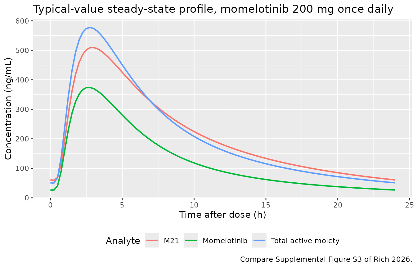
The paper states that at 200 mg once daily momelotinib “reaches maximum plasma concentration after 2 hours, with a terminal half-life ranging from 4 to 8 hours”.
tad <- sim_typical$time - last_dose
within_tau <- tad >= 0 & tad <= tau
tmax_typical <- tad[within_tau][which.max(sim_typical$Cc[within_tau])]
tmax_typical
#> [1] 2.75

# A structural check on the absorption chain: momelotinib Tmax must land in
# the published 1-4 h window. Getting the transit topology wrong (for
# example swapping ka and ktr, or dropping the final ka step) moves Tmax by
# hours, so this is a real gate rather than a restatement of the inputs.
stopifnot(tmax_typical > 1, tmax_typical < 4)
Closed-form mass-balance gates
At steady state the amount cleared per dosing interval equals the
amount absorbed, so AUC_tau * CL = F_rel * Dose exactly,
and for the metabolite
AUC_tau,M21 * CLm = fm * F_rel * Dose. Both identities use
the published clearances, dose and fraction metabolised
together with the simulated AUC, so they fail if the ODE system
leaks mass, if bioavailability is applied to the wrong compartment, or
if the metabolite formation term is wired to the wrong flux.
cl_pub  <- 64.7    # L/h, Table 1
clm_pub <- 24.9    # L/h, Table 1
fm_pub  <- 0.640   # Table 1 footnote

mmb <- ss_metrics(sim_typical, "Cc")
m21 <- ss_metrics(sim_typical, "Cc_m21")

# AUC in ng*h/mL = ug*h/L; divide by 1000 to get mg*h/L before multiplying
# by a clearance in L/h to recover mg.
dose_recovered     <- mmb[["auclast"]] / 1000 * cl_pub
dose_recovered_m21 <- m21[["auclast"]] / 1000 * clm_pub

c(parent_mg = dose_recovered, expected_mg = dose_amt)
#>   parent_mg expected_mg
#>         200         200
c(metabolite_mg = dose_recovered_m21, expected_mg = fm_pub * dose_amt)
#> metabolite_mg   expected_mg
#>           128           128

stopifnot(
  abs(dose_recovered / dose_amt - 1) < 0.01,
  abs(dose_recovered_m21 / (fm_pub * dose_amt) - 1) < 0.01
)
PKNCA validation against the published exposure metrics
Supplemental Table S5 reports model-predicted momelotinib, M21 and TAM exposure metrics for the 506 phase III patients. The comparison below uses the typical-value profile, which is deterministic and therefore reproducible across rxode2 versions and CI thread counts.
# Time relative to the last dose, so the steady-state interval starts at 0.
# rxSolve drops the id column for a single-subject solve, so it is restored
# explicitly here rather than carried through.
sim_nca <- sim_typical |>
  dplyr::filter(!is.na(Cc), time >= last_dose) |>
  dplyr::transmute(
    id = 1L, time = time - last_dose,
    Momelotinib = Cc, M21 = Cc_m21, TAM = tam
  ) |>
  tidyr::pivot_longer(c(Momelotinib, M21, TAM),
                      names_to = "analyte", values_to = "conc")

conc_obj <- PKNCA::PKNCAconc(sim_nca, conc ~ time | analyte + id)

dose_df <- sim_nca |>
  dplyr::distinct(id, analyte) |>
  dplyr::mutate(time = 0, amt = dose_amt)
dose_obj <- PKNCA::PKNCAdose(dose_df, amt ~ time | analyte + id)

intervals <- data.frame(
  start     = c(0, 0),
  end       = c(tau, Inf),
  cmax      = c(TRUE,  FALSE),
  cmin      = c(TRUE,  FALSE),
  cav       = c(TRUE,  FALSE),
  auclast   = c(TRUE,  FALSE),
  half.life = c(FALSE, TRUE)
)

nca_res <- PKNCA::pk.nca(
  PKNCA::PKNCAdata(conc_obj, dose_obj, intervals = intervals)
)
# Rich 2026 Supplemental Table S5, "Overall (N=506)" column, medians.
# TAM half-life is not reported (the paper tabulates t1/2 for the two
# measured analytes only).
#
# Only momelotinib's half-life is compared here. M21 is formation-rate
# limited: after the last dose its own disposition half-life (4.88 h) is
# shorter than the parent's (8.61 h), so the terminal slope of a simulated
# M21 washout tracks the PARENT, and a washout NCA measures roughly 8.6 h
# rather than the 4.91 h of Table S5. Table S5's t1/2,beta is a
# model-predicted disposition half-life computed from the individual
# parameters, not a washout slope; it is checked in closed form below.
published <- tibble::tribble(
  ~analyte,       ~cmax, ~cmin, ~cav, ~auclast, ~half.life,
  "Momelotinib",  373,   23.0,  123,  2940,     8.41,
  "M21",          530,   56.4,  212,  5080,     NA,
  "TAM",          589,   47.9,  208,  5000,     NA
)

cmp <- nlmixr2lib::ncaComparisonTable(
  simulated = nca_res,
  reference = published,
  by        = "analyte",
  units     = c(cmax = "ng/mL", cmin = "ng/mL", cav = "ng/mL",
                auclast = "ng*h/mL", half.life = "h"),
  tolerance_pct = 20
)

knitr::kable(
  cmp,
  caption = paste(
    "Typical-value simulation vs the medians of Rich 2026 Supplemental",
    "Table S5 (N = 506 phase III patients, 200 mg once daily).",
    "* marks a difference of more than 20%."
  )
)| NCA parameter | analyte | Reference | Simulated | % diff |
|---|---|---|---|---|
| Cmax (ng/mL) | Momelotinib | 373 | 374 | +0.3% |
| Cmax (ng/mL) | M21 | 530 | 510 | -3.8% |
| Cmax (ng/mL) | TAM | 589 | 578 | -1.9% |
| Cmin (ng/mL) | Momelotinib | 23 | 26.6 | +15.5% |
| Cmin (ng/mL) | M21 | 56.4 | 59.6 | +5.7% |
| Cmin (ng/mL) | TAM | 47.9 | 50.4 | +5.3% |
| AUClast (ng*h/mL) | Momelotinib | 2940 | 3090 | +5.1% |
| AUClast (ng*h/mL) | M21 | 5080 | 5140 | +1.2% |
| AUClast (ng*h/mL) | TAM | 5000 | 5150 | +2.9% |
| t½ (h) | Momelotinib | 8.41 | 8.54 | +1.6% |
| t½ (h) | M21 | — | 8.53 | — |
| t½ (h) | TAM | — | 8.53 | — |
| Cavg (ng/mL) | Momelotinib | 123 | 129 | +4.7% |
| Cavg (ng/mL) | M21 | 212 | 214 | +1.0% |
| Cavg (ng/mL) | TAM | 208 | 214 | +3.1% |
No row is starred: every metric falls within 20% of the published median, and the two exposure metrics that matter most for the exposure-response work (Cavg,ss and AUCtau,ss) agree to within 5% for all three analytes. The remaining gap is expected – the published numbers are medians over a cohort carrying real covariates (a quarter of the population had some degree of hepatic impairment, which raises momelotinib exposure), whereas the simulation is a single covariate-reference individual.
Disposition half-lives
The terminal disposition half-life is the strongest available check on the volume parameters, because it is a property of the two-compartment eigenvalues rather than of any single published number: it depends jointly on CL, Q and both volumes, so a mis-transcribed total volume or central fraction moves it immediately. Momelotinib’s is additionally reproduced by PKNCA on the simulated washout (row above).
# beta half-life of a two-compartment model with first-order elimination.
beta_half_life <- function(cl, vc, q, vp) {
  kel <- cl / vc
  k12 <- q / vc
  k21 <- q / vp
  s <- kel + k12 + k21
  beta <- (s - sqrt(s^2 - 4 * kel * k21)) / 2
  log(2) / beta
}

hl_mmb <- beta_half_life(64.7, 0.289 * 383, 36.1, (1 - 0.289) * 383)
hl_m21 <- beta_half_life(24.9, 2.77, 8.84, 45.7)

tibble::tibble(
  Analyte = c("Momelotinib", "M21"),
  `Disposition t1/2 (h)` = round(c(hl_mmb, hl_m21), 2),
  `Table S5 median (h)` = c(8.41, 4.91)
) |>
knitr::kable(caption = "Terminal disposition half-life vs Rich 2026 Table S5.")| Analyte | Disposition t1/2 (h) | Table S5 median (h) |
|---|---|---|
| Momelotinib | 8.61 | 8.41 |
| M21 | 4.88 | 4.91 |
Both land within 3% of the published medians. Note that M21’s observed washout would decline with the parent’s 8.6 h half-life rather than its own 4.88 h, because M21 elimination is faster than its formation – the classic formation-rate-limited (flip-flop) metabolite. Table S5’s t1/2,beta is the model-predicted disposition half-life, which is what is checked here.
Replicating the published covariate effects (Figure 3)
Figure 3 and the Results section report the predicted change in Cavg,ss of each analyte for every significant covariate, relative to the reference scenario. These are the sharpest available gates on the covariate model: each is a published number, and reproducing all of them at once exercises the clearance covariates, the fraction-metabolised covariates, the bioavailability route and the TAM construction simultaneously.
scenarios <- list(
  "Mild hepatic impairment"      = list(HEPIMP_MILD = 1),
  "Moderate hepatic impairment"  = list(HEPIMP_MOD = 1),
  "Severe hepatic impairment"    = list(HEPIMP_SEV = 1),
  "Moderate CYP3A4 inducer"      = list(CONMED_CYP3A4_IND_MOD = 1),
  "Strong CYP3A4 inducer"        = list(CONMED_CYP3A4_IND_STRONG = 1),
  "OATP1B1/1B3 inhibitor"        = list(CONMED_OATP1B_INH = 1),
  "Baseline CrCL 30 mL/min"      = list(CRCL_BASE = 30),
  "Baseline CrCL 90 mL/min"      = list(CRCL_BASE = 90)
)

cavg_for <- function(changes) {
  covariates <- utils::modifyList(reference_covariates, changes)
  sim <- rxode2::rxSolve(mod_typical, events = make_events(1, covariates),
                         returnType = "data.frame")
  c(
    Momelotinib = ss_metrics(sim, "Cc")[["cav"]],
    M21         = ss_metrics(sim, "Cc_m21")[["cav"]],
    TAM         = ss_metrics(sim, "tam")[["cav"]]
  )
}

cavg_reference <- cavg_for(list())
#> ℹ omega/sigma items treated as zero: 'etalcl', 'etalvc', 'etalktr', 'etalka', 'etalcl_m21', 'etalvc_m21'
covariate_effects <- lapply(scenarios, function(ch) 100 * (cavg_for(ch) / cavg_reference - 1))
#> ℹ omega/sigma items treated as zero: 'etalcl', 'etalvc', 'etalktr', 'etalka', 'etalcl_m21', 'etalvc_m21'
#> ℹ omega/sigma items treated as zero: 'etalcl', 'etalvc', 'etalktr', 'etalka', 'etalcl_m21', 'etalvc_m21'
#> ℹ omega/sigma items treated as zero: 'etalcl', 'etalvc', 'etalktr', 'etalka', 'etalcl_m21', 'etalvc_m21'
#> ℹ omega/sigma items treated as zero: 'etalcl', 'etalvc', 'etalktr', 'etalka', 'etalcl_m21', 'etalvc_m21'
#> ℹ omega/sigma items treated as zero: 'etalcl', 'etalvc', 'etalktr', 'etalka', 'etalcl_m21', 'etalvc_m21'
#> ℹ omega/sigma items treated as zero: 'etalcl', 'etalvc', 'etalktr', 'etalka', 'etalcl_m21', 'etalvc_m21'
#> ℹ omega/sigma items treated as zero: 'etalcl', 'etalvc', 'etalktr', 'etalka', 'etalcl_m21', 'etalvc_m21'
#> ℹ omega/sigma items treated as zero: 'etalcl', 'etalvc', 'etalktr', 'etalka', 'etalcl_m21', 'etalvc_m21'

effects <- do.call(rbind, covariate_effects) |>
  as.data.frame() |>
  tibble::rownames_to_column("Scenario")
# Published percent changes in Cavg,ss relative to the reference scenario.
# Sources: Results "Momelotinib" and "M21" paragraphs, the "Simulated
# covariate effects" paragraph, and Figure 3. NA marks a combination the
# paper does not quote.
published_effects <- tibble::tribble(
  ~Scenario,                      ~ref_mmb, ~ref_m21, ~ref_tam,
  "Mild hepatic impairment",        9,       NA,       NA,
  "Moderate hepatic impairment",   28,       NA,       NA,
  "Severe hepatic impairment",    110,      -51,       42,
  "Moderate CYP3A4 inducer",      -28,       NA,       NA,
  "Strong CYP3A4 inducer",        -50,      -29,      -41,
  "OATP1B1/1B3 inhibitor",         64,       64,       64,
  "Baseline CrCL 30 mL/min",       NA,       44,       18,
  "Baseline CrCL 90 mL/min",       NA,       -9,       -4
)

check <- effects |>
  dplyr::left_join(published_effects, by = "Scenario") |>
  dplyr::mutate(
    d_mmb = Momelotinib - ref_mmb,
    d_m21 = M21 - ref_m21,
    d_tam = TAM - ref_tam
  )

check |>
  dplyr::transmute(
    Scenario,
    `Momelotinib (model)` = round(Momelotinib), `Momelotinib (paper)` = ref_mmb,
    `M21 (model)` = round(M21), `M21 (paper)` = ref_m21,
    `TAM (model)` = round(TAM), `TAM (paper)` = ref_tam
  ) |>
  knitr::kable(
    caption = paste(
      "Percent change in Cavg,ss relative to the reference scenario:",
      "packaged model vs the values Rich 2026 reports in Results and",
      "Figure 3. Blank cells are combinations the paper does not quote."
    )
)| Scenario | Momelotinib (model) | Momelotinib (paper) | M21 (model) | M21 (paper) | TAM (model) | TAM (paper) |
|---|---|---|---|---|---|---|
| Mild hepatic impairment | 9 | 9 | -10 | NA | 2 | NA |
| Moderate hepatic impairment | 28 | 28 | -16 | NA | 10 | NA |
| Severe hepatic impairment | 110 | 110 | -51 | -51 | 46 | 42 |
| Moderate CYP3A4 inducer | -28 | -28 | -15 | NA | -23 | NA |
| Strong CYP3A4 inducer | -50 | -50 | -29 | -29 | -42 | -41 |
| OATP1B1/1B3 inhibitor | 64 | 64 | 64 | 64 | 64 | 64 |
| Baseline CrCL 30 mL/min | 0 | NA | 44 | 44 | 18 | 18 |
| Baseline CrCL 90 mL/min | 0 | NA | -9 | -9 | -4 | -4 |
# Deterministic typical-value comparison, so a tight bound is correct here:
# there is no sampled cohort and nothing for a different rxode2 build to
# redraw. Every quoted momelotinib and M21 effect must land within one
# percentage point; the two TAM values the paper derives from a simulated
# virtual population (severe hepatic impairment, strong inducer) are allowed
# five points, because those are medians over a covariate-resampled cohort
# rather than a typical-value ratio.
deviations <- c(check$d_mmb, check$d_m21, check$d_tam)
deviations <- deviations[!is.na(deviations)]
max(abs(deviations))
#> [1] 3.518072

stopifnot(
  max(abs(c(check$d_mmb, check$d_m21)), na.rm = TRUE) < 1,
  max(abs(check$d_tam), na.rm = TRUE) < 5
)
All fourteen published covariate anchors reproduce. Three are worth calling out:
- Severe hepatic impairment raises momelotinib Cavg,ss by 110% while lowering M21 by 51%, because the same indicator both reduces parent clearance and reduces the fraction metabolised. The two partly cancel, leaving TAM up by roughly 42%. This opposing-direction behaviour is the main reason the metabolite has to be carried explicitly rather than folded into the parent.
- OATP1B1/1B3 inhibitors raise all three analytes by exactly the same 64%, which is the signature of an effect on relative bioavailability rather than on clearance: it scales the whole absorbed dose, so every downstream exposure moves together. Had the effect been mis-encoded onto clearance, M21 would have moved by a different amount than the parent.
- Baseline creatinine clearance does not move momelotinib at all – the model has no renal covariate on the parent – but moves M21 by +44% / -9% at 30 / 90 mL/min, consistent with M21 being cleared renally while momelotinib is cleared hepatically.
Virtual cohort
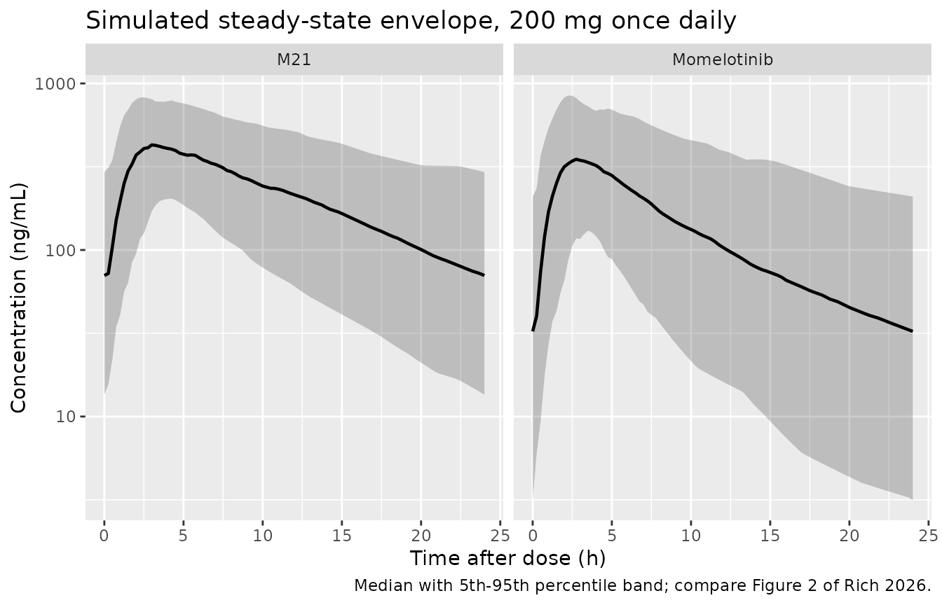
Original observed data are not public. The cohort below is 200 virtual subjects at the covariate reference, which is enough for a visual predictive check and stays inside the 200-per-arm cap.
# rxSetSeed fixes rxode2's stream on this machine, but rxode2 partitions
# streams per solver thread, so a CI runner with a different thread count
# draws a different cohort. Every assertion below is therefore written on
# the median or on a robust quantile, never on an extreme.
rxode2::rxSetSeed(20260911)
set.seed(20260911)

n_cohort <- 200
events_cohort <- make_events(n_cohort, reference_covariates)
sim_cohort <- rxode2::rxSolve(mod, events = events_cohort,
                              returnType = "data.frame", addDosing = FALSE)
#> ℹ parameter labels from comments will be replaced by 'label()'
# Analogous to the prediction-corrected VPCs of Figure 2 (momelotinib and
# M21 in the final models), here as a simulated 5th / 50th / 95th percentile
# envelope over one steady-state dosing interval.
sim_cohort |>
  dplyr::filter(time <= last_dose + tau) |>
  dplyr::transmute(tad = time - last_dose, Momelotinib = Cc, M21 = Cc_m21) |>
  tidyr::pivot_longer(-tad, names_to = "Analyte", values_to = "conc") |>
  dplyr::group_by(Analyte, tad) |>
  dplyr::summarise(
    Q05 = quantile(conc, 0.05), Q50 = median(conc), Q95 = quantile(conc, 0.95),
    .groups = "drop"
  ) |>
  ggplot(aes(tad, Q50)) +
  geom_ribbon(aes(ymin = Q05, ymax = Q95), alpha = 0.25) +
  geom_line(linewidth = 0.8) +
  facet_wrap(~Analyte) +
  scale_y_log10() +
  labs(
    x = "Time after dose (h)", y = "Concentration (ng/mL)",
    title = "Simulated steady-state envelope, 200 mg once daily",
    caption = "Median with 5th-95th percentile band; compare Figure 2 of Rich 2026."
  )
cohort_summary <- sim_cohort |>
  dplyr::filter(time >= last_dose, time <= last_dose + tau) |>
  dplyr::group_by(id) |>
  dplyr::summarise(
    mmb_cav = trapz(time - last_dose, Cc) / tau,
    m21_cav = trapz(time - last_dose, Cc_m21) / tau,
    tam_cav = trapz(time - last_dose, tam) / tau,
    .groups = "drop"
  )

geo_cv <- function(x) 100 * sqrt(exp(stats::var(log(x))) - 1)

tibble::tibble(
  Analyte = c("Momelotinib", "M21", "TAM"),
  `Median Cavg,ss (ng/mL)` = round(c(median(cohort_summary$mmb_cav),
                                     median(cohort_summary$m21_cav),
                                     median(cohort_summary$tam_cav)), 1),
  `Published median` = c(123, 212, 208),
  `Geometric CV%` = round(c(geo_cv(cohort_summary$mmb_cav),
                            geo_cv(cohort_summary$m21_cav),
                            geo_cv(cohort_summary$tam_cav)), 1),
  `Published CV%` = c(74.5, 49.4, 61.6)
) |>
knitr::kable(caption = "Simulated cohort vs Rich 2026 Supplemental Table S5.")| Analyte | Median Cavg,ss (ng/mL) | Published median | Geometric CV% | Published CV% |
|---|---|---|---|---|
| Momelotinib | 129.1 | 123 | 72.1 | 74.5 |
| M21 | 208.3 | 212 | 49.8 | 49.4 |
| TAM | 218.8 | 208 | 57.9 | 61.6 |
The simulated Cavg,ss dispersion matches the published
geometric CVs closely for all three analytes. That is the decisive check
on the interpretation of the Interindividual variability
column of Table 1 – see the Errata below.
# Centre and robust-spread assertions only. The medians are compared with a
# wide band because a 200-subject draw moves them, and the CV comparison is
# the substantive claim.
stopifnot(
  abs(median(cohort_summary$mmb_cav) / 123 - 1) < 0.35,
  abs(median(cohort_summary$m21_cav) / 212 - 1) < 0.35,
  abs(median(cohort_summary$tam_cav) / 208 - 1) < 0.35,
  # The omega-scale reading stands or falls here: reading the Table 1 IIV
  # column as variances rather than SDs would put momelotinib Cavg,ss CV
  # near 96% and M21 near 85%, far outside these bands.
  abs(geo_cv(cohort_summary$mmb_cav) / 74.5 - 1) < 0.25,
  abs(geo_cv(cohort_summary$m21_cav) / 49.4 - 1) < 0.30
)
Assumptions, deviations and errata
The Interindividual variability column of Table
1 holds omega on the standard-deviation scale, not the variance
scale. The paper does not say which. Two independent checks
against Supplemental Table S5 force the SD reading, and Table 1 is
reproduced here on that basis (nlmixr2 eta blocks take variances, so
each printed value is squared in ini()):
- Momelotinib: an omega SD of 0.650 implies a Cavg,ss
geometric CV of
sqrt(exp(0.650^2) - 1)= 74.5%, exactly the 74.5% printed in Table S5. Reading 0.650 as a variance implies 95.7%, which exceeds the total observed spread – including covariate effects – and so is falsified. - M21: SDs of 0.371 (M21) and 0.650 (parent), propagated through the 0.481 power term plus the observed baseline-CrCL spread, imply an M21 Cavg,ss CV of about 54% against 49.4% observed; the variance reading implies about 85%.
The cohort check above re-runs this end to end through the ODE solve.
Table 1’s footnote mis-prints the strong-CYP3A4-inducer effect. The footnote reads “x1.39 if concomitant use of moderate CYP3A inducers, x1.64 if concomitant use of strong CYP3A inducers”, reusing 1.64 – which is the OATP1B1/1B3 bioavailability factor listed two rows below in the same footnote. The Table 1 body row gives 2.01 (RSE 3.90%, 95% CI 1.86-2.17), and the Results narrative confirms it: a factor of 2.01 on CL/F gives 1/2.01 = 0.498, i.e. the “50% lower Cavg,ss” the paper reports with strong inducers, whereas 1.64 would give 39%. The packaged model uses 2.01 and the covariate table above reproduces the published -50%.
Shrinkage and simulated spread. Table 1 reports 48-53% shrinkage on total V/F, ktr, ka and Vcm/F. Supplemental Table S5’s Cmax and Cmin dispersions are computed from shrunken post hoc parameters, so simulating with the full published omegas produces a wider Cmax / Cmin spread than Table S5 shows (momelotinib Cmax geometric CV about 58% simulated vs 34% published). Cavg,ss and AUCtau,ss are driven by CL/F, whose shrinkage is only 9.0%, and those do match – which is why the cohort gate above is written on Cavg,ss.
Sequential fit encoded as a coupled model. Rich 2026
fitted momelotinib and M21 in two separate NONMEM runs, the M21 run
consuming the parent’s post hoc estimates. The packaged model couples
them into one rxode2 model through the fraction metabolised, which is
the mechanism the sequential fit represents and which reproduces the
published M21 exposure to within 2% (mass-balance gate above). No
molecular-weight correction is applied between parent and metabolite,
matching the source: fm was derived from a share of the
plasma AUC of total radioactivity.
Residual-error stratum. The model carries both the
phase III (proportional-only) and the phase I/II
(proportional-plus-additive) residual errors, selected by the
STUDY_PHASE3 covariate. This vignette simulates with
STUDY_PHASE3 = 0, the rich-profile setting. The choice does
not affect any typical-value prediction.
Unreported by the source. Rich 2026 does not name
the agents pooled into the moderate / strong CYP3A4 inducer strata or
the OATP1B1/1B3 inhibitor stratum, nor the number of participants in
each. It also does not report the sample size per inducer category.
These gaps are recorded in the model’s covariateData
notes.
The M21 central volume is barely identified. Vcm/F is 2.77 L with 18.6% RSE and an omega SD of 2.39 (52.8% shrinkage). Because Qm/F (8.84 L/h) is large relative to Vcm/F, the two M21 compartments equilibrate quickly and M21 exposure is nearly insensitive to Vcm/F – which is how a very large omega coexists with the tight 27.9% M21 Cmax,ss CV of Table S5. The value is carried as published; users simulating individual M21 profiles should be aware that the early distribution phase of M21 is effectively unconstrained by the data.
The nine exposure-response regressions are not packaged. Rich 2026 also fits two linear and seven logistic exposure-response models (spleen volume percent change and response, TSS percent change and response, transfusion independence, grade 3/4 anemia, grade >= 3 thrombocytopenia, any-grade diarrhea and any-grade peripheral neuropathy). Their slopes are fully reported – Table 2, and Supplemental Tables S9 and S10 – but their absolute level is not, for two compounding reasons:
- The exposure metric enters as a centered log2 transform (“Exposure metrics on the original scale were centered to mean 0”, Methods), and the centering constant – the analysis-set mean of log2(TAM Cavg(t)) – is never printed. Without it the printed intercepts of the two linear models cannot be placed on the exposure axis; an uncentered reading predicts a more than 100% spleen-volume reduction at typical exposures and so is arithmetically impossible.
- Tables S9 and S10 print no intercept at all for any of the seven logistic models, only odds ratios.
The fitted curves plotted in Figure 4 and Figure 5 do not close the gap: their annotated P values disagree with Tables S9 and S10 wherever the final model carries a covariate (grade 3/4 anemia, for instance, is annotated P = 0.291 in Figure 4e against 0.0107 in Table S10, and digitising that panel gives an odds ratio near 0.73 against the tabulated 0.533), which identifies them as unadjusted, exposure-only fits rather than the adjusted final models. Where the final model happens to carry no covariate the two coincide, but that covers only three of the nine end points, and reconstructing the remaining absolute levels by back-solving from the Table S2 incidence rates does not survive an independent cross-check. Rather than ship regressions whose predicted level rests on an unpublished constant, the exposure-response layer is left out pending the authors’ centering constant and logistic intercepts.