Ethinylestradiol (Ezuruike 2018)
Source:vignettes/articles/Ezuruike_2018_ethinylestradiol.Rmd
Ezuruike_2018_ethinylestradiol.RmdModel and source
- Citation: Ezuruike U, Humphries H, Dickins M, Neuhoff S, Gardner I, Rowland Yeo K. (2018). Risk-Benefit Assessment of Ethinylestradiol Using a Physiologically Based Pharmacokinetic Modeling Approach. Clin Pharmacol Ther 104(6):1229-1239. doi:10.1002/cpt.1085. Includes the publisher’s correction of 11 May 2018 to Table 2.
- Article: https://doi.org/10.1002/cpt.1085 (PMC6282492, open access)
- Supplement (Tables S1-S2, Figures S1-S2): published with the article, https://europepmc.org/article/PMC/PMC6282492
Ethinylestradiol (EE) is the estrogen component of almost every combined oral contraceptive. Ezuruike 2018 built a minimal distribution PBPK model with a single adjusting compartment (SAC) in the Simcyp Population-based Simulator (V17r1) in order to (i) resolve how much of EE’s clearance really runs through CYP3A4, and (ii) ask how often a woman’s steady-state EE exposure falls outside a therapeutic window when a CYP-modulating drug is co-prescribed.
What this model file is, and what it is not
This is a reduction of the published Simcyp model, not a port of it. The whole-body mass-balance equations and the virtual-population database are not published and cannot be encoded here.
What is published is enough to rebuild the disposition exactly, with no fitted parameters:
- Table 4 [Table 3 in print is a different table; see the note on
table numbering below] gives the whole compound layer –
fa,ka,Qgut,fu,gut,Vss, the SACKin/Kout, and the renal clearance; - the Results give the gut and hepatic extraction ratios
(
EG= 0.44,EH= 0.25) measured by simultaneous portal-vein and systemic sampling; - Figure 3b gives the final optimized model’s own predicted split of systemic elimination across CYP3A4, CYP2C9, CYP1A2, CYP2C8, UGT1A1, the unassigned “additional HLM” pathways, and renal clearance.
Those three sources pin every parameter in the file. Each coadministered CYP modulator then enters through a single relative CYP3A4 activity term that scales gut-wall intrinsic clearance, hepatic intrinsic clearance and systemic clearance together; each activity is back-solved from that arm’s published AUC ratio alone, leaving the published Cmax ratios as a genuine hold-out.
What is not reproducible, and is therefore absent:
- the Simcyp virtual-population variability. The paper reports only
ranges of trial means, never a variance component, so this is a
typical-value model: no etas,
propSdfixed at 0. The counts of virtual subjects crossing the paper’s exposure thresholds therefore cannot be reproduced – the population means behind them can, and all fifteen of them are checked below; - the perpetrator models themselves. The authors built a voriconazole
compound model (supplementary Table S2) and took the other perpetrators
from the Simcyp V17 compound library; the interaction runs on
time-varying perpetrator concentrations against published
Ki/Indmaxvalues inside the platform. None of that is needed here, because the paper prints the resulting exposure ratios and those are what the model encodes.
A note on table numbering
The article’s tables are numbered 1-4 in the PDF, but the print layout labels the risk-benefit grid “Table 3” and the compound-input table “Table 4” while the running text refers to the risk-benefit grid as Table 3. Throughout this vignette, “Table 4 [Table 3 in print]” means the five-column grid of steady-state AUC by dose and CYP-modulation scenario, and “Table 4 (inputs)” means the compound-parameter table. The model file’s source-trace comments use the same convention.
Population
- Species: human
- Reference simulation: 100 virtual subjects (10 trials x 10 healthy female volunteers, 20-50 years)
- Sex: 100% female
- Doses: Ethinylestradiol 20, 35 and 50 ug once daily by mouth (and a single 50 ug intravenous dose for the distribution fit).
- Virtual population: Simcyp healthy-volunteer virtual population, trial-matched demographics.
Every simulation in the paper was matched to the demographics of the clinical study it reproduced (supplementary Table S1): voriconazole n = 16 aged 18-40, fluconazole n = 21 aged 18-36, carbamazepine n = 10 aged 18-40 and n = 10 aged 18-35, rifampicin n = 22 aged 18-45 and n = 12 aged 23-44. The reference control simulation, and every cell of the risk-benefit grid, used 10 trials of 10 healthy women aged 20-50.
Source trace
Every value in ini(), and where it comes from.
| Parameter | Value | Source location |
|---|---|---|
| lka | log(1.103) 1/h | Table 4 (inputs), ‘ka (1/h)’; Simcyp-predicted from PSA / HBD |
| fa | 0.948 | Table 4 (inputs), ‘fa’; Figure 3a rounds it to ‘Fa = 1’ |
| lvc | log(71.2355) L | Derived: Vss 4.06 L/kg (Table 4 inputs) x 70 kg / (1 + Kin/Kout) |
| lk12 | log(0.287) 1/h | Table 4 (inputs), ‘K in’ (unit column reads L/h; see Errata) |
| lk21 | log(0.096) 1/h | Table 4 (inputs), ‘K out’ (same unit note) |
| lcl_renal | log(2.079) L/h | Table 4 (inputs), ‘CL R (L/h)’; Results derive it as 6% of CL/F 34.6 L/h |
| lcl_nonren | log(9.9831) L/h | Derived: CLR / 0.172359 - CLR, using the 17.26% renal slice of Figure 3b |
| eh | 0.25 | Results ‘First-pass metabolism’: EH = 0.25 (Back et al. 1982) |
| qgut | 11.74 L/h | Table 4 (inputs), ‘Q gut (L/h)’ |
| lcl_int_g_cyp3a4 | log(2.5184) L/h | Derived: Qgut x EG / (1 - EG) x 0.40 x 22.19/(22.19 + 10.32) |
| lcl_int_g_cyp2c9 | log(1.1713) L/h | Derived: same total x 0.40 x 10.32/(22.19 + 10.32) |
| lcl_int_g_other | log(5.5346) L/h | Derived: same total x 0.60 (sulfation + glucuronidation) |
| fm_cyp3a4 | 0.26774 | Figure 3b, 22.19% / 82.88% (non-renal slices) |
| fm_cyp2c9 | 0.12452 | Figure 3b, 10.32% / 82.88% |
| fm_cyp1a2 | 0.08711 | Figure 3b, 7.22% / 82.88% |
| fm_cyp2c8 | 0.01279 | Figure 3b, 1.06% / 82.88% |
| fm_ugt1a1 | 0.06322 | Figure 3b, 5.24% / 82.88% |
| fm_other | 0.44462 | Figure 3b, 36.85% / 82.88% (‘additional HLM’) |
| e_conmed_ketoconazole_cyp3a4 | log(0.2223) | Back-solved from AUC ratio 1.347, Table 4 [Table 3 in print] |
| e_conmed_voriconazole_cyp3a4 | log(0.1314) | Back-solved from predicted AUC ratio 1.40, Table 1 |
| e_conmed_fluconazole_cyp3a4 | log(0.6655) | Back-solved from predicted AUC ratio 1.13, Table 1 |
| e_conmed_cbz_cyp3a4 | log(2.6055) | Back-solved from predicted AUC ratio 0.61, Table 1 |
| e_conmed_efv_cyp3a4 | log(2.5796) | Back-solved from AUC ratio 0.614, Table 4 [Table 3 in print] |
| e_conmed_rifampicin_cyp3a4 | log(4.8546) | Back-solved from predicted AUC ratio 0.36 (600 mg QD), Table 1 |
| e_dose_rifampicin_cyp3a4 | log(4.8546/4.3542) | 300 mg QD arm gives 4.3542 from AUC ratio 0.40, Table 1 |
| propSd | 0 (fixed) | No residual-error model is reported |
The three derived quantities, spelled out
Only three numbers in the file are not transcribed directly. Each is an arithmetic consequence of printed values, reproduced here in code.
# 1. Central volume. Table 4 (inputs) gives Vss = 4.06 L/kg and SAC transfer
#    constants Kin / Kout that act on drug MASS, so at steady state the SAC holds
#    Kin/Kout times the systemic amount.
bw <- 70                         # reference body weight; see Errata
vss_total <- 4.06 * bw
vc_derived <- vss_total / (1 + 0.287 / 0.096)

# 2. Systemic clearance. Figure 3b's renal slice is 17.26% of a pie whose slices
#    sum to 100.14% as printed, so renormalise before dividing.
pie_pct <- c(cyp3a4 = 22.19, cyp2c9 = 10.32, cyp1a2 = 7.22, cyp2c8 = 1.06,
             ugt1a1 = 5.24, other = 36.85, renal = 17.26)
pie <- pie_pct / sum(pie_pct)
cl_renal <- 2.079
cl_total <- cl_renal / pie[["renal"]]
cl_nonren <- cl_total - cl_renal

# 3. Gut-wall intrinsic clearance, from the printed Qgut and gut availability.
qgut <- 11.74
fg <- 0.56
clint_g_total <- qgut * (1 - fg) / fg
hydroxylation_share <- 0.40      # 20% pre-refinement, doubled by the CYP refinement
cyp3a4_of_hydrox <- pie_pct[["cyp3a4"]] / (pie_pct[["cyp3a4"]] + pie_pct[["cyp2c9"]])

data.frame(
  Quantity = c("vc (L)", "CL total (L/h)", "CL non-renal (L/h)",
               "CLint,G total (L/h)", "CLint,G CYP3A4 (L/h)",
               "CLint,G CYP2C9 (L/h)", "CLint,G other (L/h)",
               "baseline EG re-derived", "baseline F"),
  Value = round(c(
    vc_derived, cl_total, cl_nonren, clint_g_total,
    clint_g_total * hydroxylation_share * cyp3a4_of_hydrox,
    clint_g_total * hydroxylation_share * (1 - cyp3a4_of_hydrox),
    clint_g_total * (1 - hydroxylation_share),
    clint_g_total / (qgut + clint_g_total),
    0.948 * fg * (1 - 0.25)
  ), 4)
)
#>                 Quantity   Value
#> 1                 vc (L) 71.2355
#> 2         CL total (L/h) 12.0621
#> 3     CL non-renal (L/h)  9.9831
#> 4    CLint,G total (L/h)  9.2243
#> 5   CLint,G CYP3A4 (L/h)  2.5184
#> 6   CLint,G CYP2C9 (L/h)  1.1713
#> 7    CLint,G other (L/h)  5.5346
#> 8 baseline EG re-derived  0.4400
#> 9             baseline F  0.3982
The re-derived gut extraction ratio returns the published 0.44 exactly, and the baseline bioavailability of 0.398 is consistent with the “F ~ 50%” of Figure 3a and with the Results’ statement that oral bioavailability is less than 50%.
Why the systemic clearance is 12.06 L/h and not the 16.47 L/h in the text. The Results quote a mean intravenous clearance of 16.47 L/h, but that literature value was the target of the retrograde calculation that produced the model’s initial hepatic intrinsic clearance, before the ketoconazole refinement raised every CYP CLint. What Figure 3b describes is the final optimized model, and its 17.26% renal share combined with the fixed 2.079 L/h renal clearance pins the final total at 12.06 L/h. Using 16.47 L/h instead would under-predict every cell of the risk-benefit grid by about 26%; using 12.06 L/h reproduces all fifteen to within 2.6%, which is the check run below.
Simulation helper
mod <- ui   # the rxUi built from readModelDb() in the chunk above

covs_none <- list(
  CONMED_KETOCONAZOLE = 0, CONMED_PANCYP_INH = 0, CONMED_VORICONAZOLE = 0,
  CONMED_FLUCONAZOLE = 0, CONMED_CBZ = 0, CONMED_EFV = 0,
  CONMED_RIFAMPICIN = 0, DOSE_RIFAMPICIN_MG = 0
)

# Multiple-dose steady-state profile for one arm. Doses are in ug, Cc in pg/mL.
simSteadyState <- function(dose_ug, cov = list(), n_days = 21, tau = 24,
                           grid_by = 0.05) {
  cv <- utils::modifyList(covs_none, cov)
  ev <- rxode2::et(amt = dose_ug, cmt = "depot", ii = tau, until = tau * (n_days - 1))
  ev <- rxode2::et(ev, seq(0, tau * n_days, by = grid_by))
  dat <- as.data.frame(ev)
  for (nm in names(cv)) dat[[nm]] <- cv[[nm]]
  rxode2::rxSolve(mod, dat, returnType = "data.frame", atol = 1e-12, rtol = 1e-10)
}

# Summary of the final dosing interval.
lastInterval <- function(sim, n_days = 21, tau = 24) {
  l <- sim[sim$time >= tau * (n_days - 1) & !is.na(sim$Cc), ]
  data.frame(
    auc_tau = sum(diff(l$time) * (utils::head(l$Cc, -1) + utils::tail(l$Cc, -1)) / 2),
    cmax = max(l$Cc),
    cmin = min(l$Cc),
    tmax = l$time[which.max(l$Cc)] - tau * (n_days - 1)
  )
}
Replicating Figure 1a: 35 ug once daily for 21 days
sim35 <- simSteadyState(35)

ggplot(sim35[!is.na(sim35$Cc), ], aes(time / 24, Cc)) +
  geom_line(linewidth = 0.6) +
  labs(x = "Time (days)", y = "Ethinylestradiol (pg/mL)") +
  theme_bw()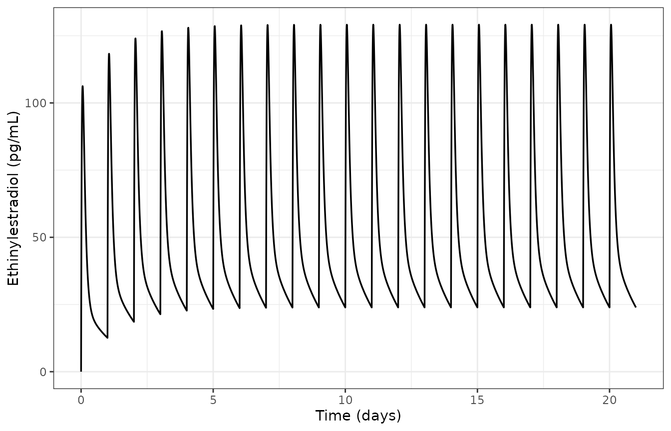
Replicates Figure 1a of Ezuruike 2018: simulated mean plasma ethinylestradiol after 35 ug once daily for 21 days.
| Metric | Simulated | Ezuruike 2018 predicted | % difference |
|---|---|---|---|
| Cmax (pg/mL) | 129.13 | 125 | 3.3 |
| AUC(0-24) (pg*h/mL) | 1155.28 | 1140 | 1.3 |
| Tmax (h) | 1.40 | NA | NA |
The paper also lists the observed day-21 values from three clinical studies: Cmax 87, 143 and 117 pg/mL and AUC(0-24) 1080, 1199 and 1062 pg*h/mL. The simulated values sit inside both observed ranges.
Replicating Figure 2: single 50 ug dose, intravenous and oral
Figure 2 of the paper shows a single 50 ug dose given intravenously (panels a, b) and orally (panels c, d). The intravenous arm is the one the SAC was fitted to, so it is the sharpest test of the distribution parameters.
# Dense early sampling: an intravenous bolus profile falls by an order of
# magnitude in the first hour, and a coarse grid biases the trapezoidal AUC.
grid_sd <- sort(unique(c(
  seq(0, 2, by = 0.01), seq(2, 24, by = 0.1), seq(24, 336, by = 0.5)
)))

simSingle <- function(arm) {
  cmt <- if (arm == "intravenous") "central" else "depot"
  ev <- rxode2::et(amt = 50, cmt = cmt)
  ev <- rxode2::et(ev, grid_sd)
  dat <- as.data.frame(ev)
  for (nm in names(covs_none)) dat[[nm]] <- covs_none[[nm]]
  out <- rxode2::rxSolve(mod, dat, returnType = "data.frame", atol = 1e-12, rtol = 1e-10)
  out$arm <- arm
  out$id <- 1L
  out
}

sim_sd <- dplyr::bind_rows(simSingle("intravenous"), simSingle("oral"))

# rxSolve() does not return the event columns, so the dose records for PKNCA are
# built from the regimen directly rather than recovered from the solve.
# `route` is a reserved PKNCA dose attribute, so the treatment grouping variable
# is called `arm` and `route` carries the value PKNCA expects.
dose_sd <- data.frame(
  id = 1L,
  time = 0,
  amt = 50,
  arm = c("intravenous", "oral"),
  route = c("intravascular", "extravascular"),
  stringsAsFactors = FALSE
)
panels <- dplyr::bind_rows(
  transform(sim_sd[!is.na(sim_sd$Cc) & sim_sd$time <= 48, ], panel = "linear scale"),
  transform(sim_sd[!is.na(sim_sd$Cc) & sim_sd$time > 0 & sim_sd$time <= 48, ],
            panel = "logarithmic scale")
)

ggplot(panels, aes(time, Cc, colour = arm)) +
  geom_line(linewidth = 0.6) +
  facet_wrap(~panel, scales = "free_y") +
  labs(x = "Time (h)", y = "Ethinylestradiol (pg/mL)", colour = NULL) +
  theme_bw() + theme(legend.position = "top")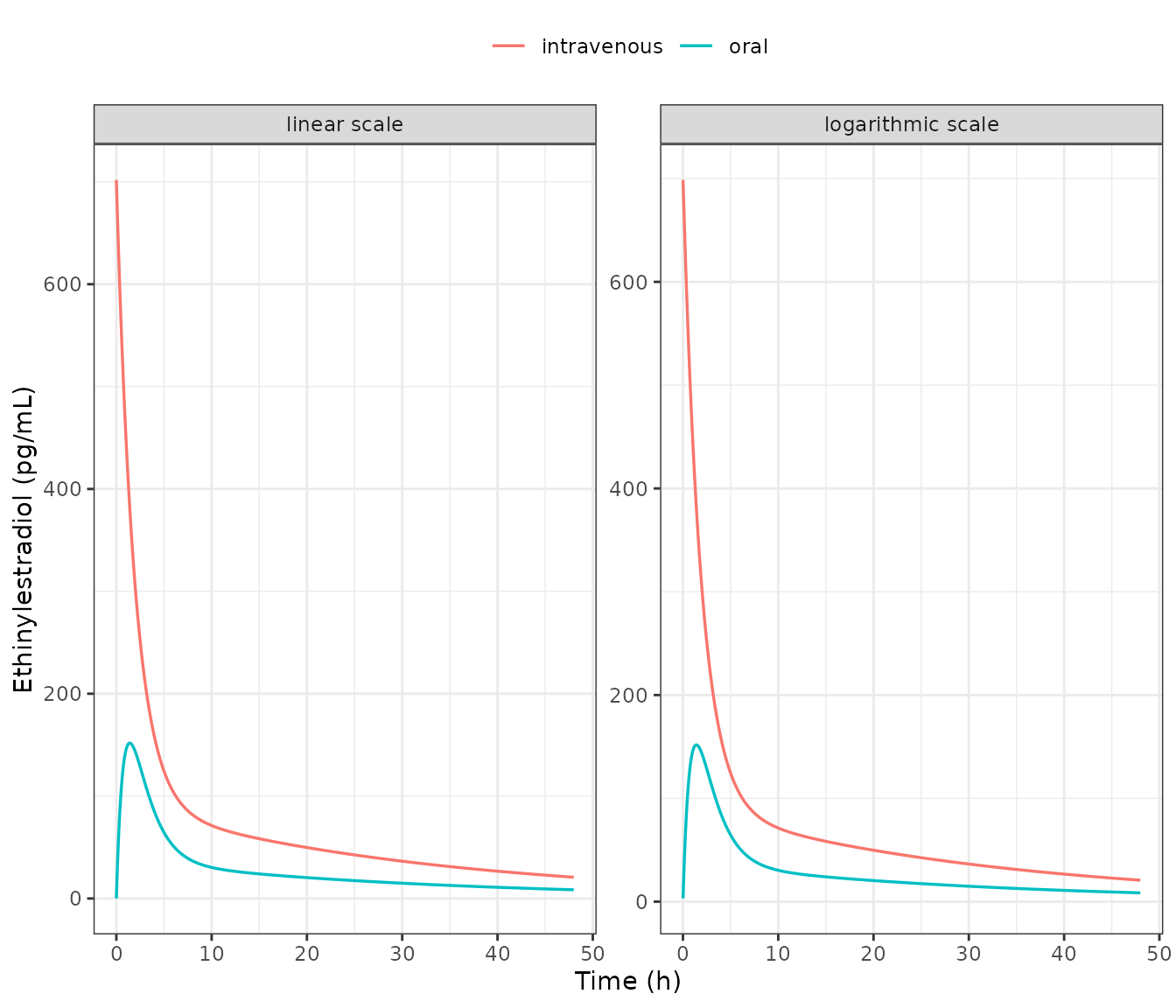
Replicates Figure 2a-d of Ezuruike 2018: single 50 ug dose given intravenously and orally, on linear and logarithmic concentration scales.
PKNCA validation
The single-dose arms are analysed with PKNCA. The intravenous arm is
a closed-form gate: non-compartmental analysis of an intravenous bolus
must return the model’s own clearance and steady-state volume, and the
latter is the value the paper prints as an input
(Vss = 4.06 L/kg). The oral arm then recovers the
bioavailability that the three printed first-pass factors imply.
nca_conc <- sim_sd |>
  dplyr::filter(!is.na(Cc)) |>
  dplyr::select(id, time, Cc, arm)

# A time-zero record must be present for every subject/arm, otherwise PKNCA
# warns that the requested AUC window starts before the first measurement.
nca_conc <- nca_conc |>
  dplyr::bind_rows(
    nca_conc |>
      dplyr::group_by(id, arm) |>
      dplyr::summarise(time = 0, Cc = 0, .groups = "drop") |>
      dplyr::select(id, time, Cc, arm)
  ) |>
  dplyr::distinct(id, arm, time, .keep_all = TRUE) |>
  dplyr::arrange(arm, time)

nca_dose <- dose_sd

# PKNCA's grouping convention puts the SUBJECT last, after the slash, and the
# treatment grouping before it, so per-arm results can be compared with the paper.
conc_obj <- PKNCA::PKNCAconc(nca_conc, Cc ~ time | arm / id)
# PKNCAdose() does not accept a nested (slash) grouping, so the dose side uses
# the same grouping variables joined with '+'.
dose_obj <- PKNCA::PKNCAdose(nca_dose, amt ~ time | arm + id)
#> Found column named route, using it for the attribute of the same name.

intervals <- data.frame(
  start = 0, end = Inf,
  cmax = TRUE, tmax = TRUE, auclast = TRUE, aucinf.obs = TRUE,
  aumcinf.obs = TRUE, half.life = TRUE, aucpext.obs = TRUE
)

nca_res <- PKNCA::pk.nca(PKNCA::PKNCAdata(conc_obj, dose_obj, intervals = intervals))

nca_wide <- as.data.frame(nca_res) |>
  dplyr::select(arm, PPTESTCD, PPORRES) |>
  tidyr::pivot_wider(names_from = PPTESTCD, values_from = PPORRES)
# Cc is in pg/mL, so AUC is in pg*h/mL; 1 pg/mL = 1e-3 ug/L, hence
# CL (L/h) = dose (ug) / (AUC * 1e-3).
iv <- nca_wide[nca_wide$arm == "intravenous", ]
po <- nca_wide[nca_wide$arm == "oral", ]

cl_nca <- 50 / (iv$aucinf.obs * 1e-3)
mrt_nca <- iv$aumcinf.obs / iv$aucinf.obs
vss_nca <- cl_nca * mrt_nca
f_nca <- po$aucinf.obs / iv$aucinf.obs

gate <- tibble::tibble(
  Quantity = c("CL from IV NCA (L/h)", "Vss from IV NCA (L)", "Vss from IV NCA (L/kg)",
               "Oral bioavailability F", "Extrapolated AUC, IV (%)"),
  `NCA of the simulation` = round(c(cl_nca, vss_nca, vss_nca / bw, f_nca, iv$aucpext.obs), 4),
  `Model input / expectation` = round(c(cl_total, vss_total, 4.06, 0.948 * fg * 0.75, NA), 4)
)
gate$`% difference` <- round(100 * (gate$`NCA of the simulation` /
                                      gate$`Model input / expectation` - 1), 2)
knitr::kable(gate, caption = paste(
  "Closed-form gate. The intravenous arm must return the model's clearance and",
  "the 4.06 L/kg steady-state volume that Ezuruike 2018 Table 4 (inputs) prints;",
  "the oral arm must return fa x (1 - EG) x (1 - EH)."
))| Quantity | NCA of the simulation | Model input / expectation | % difference |
|---|---|---|---|
| CL from IV NCA (L/h) | 12.0619 | 12.0621 | 0 |
| Vss from IV NCA (L) | 284.1947 | 284.2000 | 0 |
| Vss from IV NCA (L/kg) | 4.0599 | 4.0600 | 0 |
| Oral bioavailability F | 0.3982 | 0.3982 | 0 |
| Extrapolated AUC, IV (%) | 0.0020 | NA | NA |
stopifnot(
  abs(cl_nca / cl_total - 1) < 0.01,
  abs(vss_nca / vss_total - 1) < 0.02,
  abs(f_nca / (0.948 * fg * 0.75) - 1) < 0.01
)
The steady-state volume recovered from the simulated intravenous
profile is the 4.06 L/kg the paper prints, which confirms that the Table
4 Vss is the whole-body steady-state
volume rather than the systemic compartment alone – the reading the
model file adopts when it derives vc.
| arm | Cmax (pg/mL) | Tmax (h) | AUC0-inf (pg*h/mL) | t1/2 (h) |
|---|---|---|---|---|
| intravenous | 701.90 | 0.00 | 4145.3 | 22.15 |
| oral | 151.78 | 1.41 | 1650.5 | 22.15 |
The terminal half-life of about 22 h sits at the top of the 10-20 h
usually quoted for ethinylestradiol; it is a consequence of the
published Vss, Kin and Kout, not
a choice made here.
Comparison against the published risk-benefit grid
This is the paper’s headline table: population-mean steady-state AUC for three doses under five CYP-modulation scenarios. All fifteen cells are reproduced.
scenarios <- list(
  `Control` = list(),
  `CYP3A4 inhibition` = list(CONMED_KETOCONAZOLE = 1),
  `Complete CYP inhibition` = list(CONMED_PANCYP_INH = 1),
  `Strong CYP3A4 induction` = list(CONMED_RIFAMPICIN = 1, DOSE_RIFAMPICIN_MG = 600),
  `Moderate CYP3A4 induction` = list(CONMED_EFV = 1)
)
doses <- c(20, 35, 50)

grid_sim <- expand.grid(dose = doses, scenario = names(scenarios),
                        stringsAsFactors = FALSE)
grid_sim$auc_ss <- vapply(
  seq_len(nrow(grid_sim)),
  function(i) {
    lastInterval(simSteadyState(grid_sim$dose[i], scenarios[[grid_sim$scenario[i]]]))$auc_tau
  },
  numeric(1)
)

published <- tibble::tribble(
  ~dose, ~scenario,                    ~published,
  20L,   "Control",                     670,
  20L,   "CYP3A4 inhibition",           902,
  20L,   "Complete CYP inhibition",    1169,
  20L,   "Strong CYP3A4 induction",     244,
  20L,   "Moderate CYP3A4 induction",   412,
  35L,   "Control",                    1172,
  35L,   "CYP3A4 inhibition",          1579,
  35L,   "Complete CYP inhibition",    2046,
  35L,   "Strong CYP3A4 induction",     427,
  35L,   "Moderate CYP3A4 induction",   720,
  50L,   "Control",                    1675,
  50L,   "CYP3A4 inhibition",          2256,
  50L,   "Complete CYP inhibition",    2923,
  50L,   "Strong CYP3A4 induction",     609,
  50L,   "Moderate CYP3A4 induction",  1029
)

grid_cmp <- grid_sim |>
  dplyr::mutate(dose = as.integer(dose)) |>
  dplyr::left_join(published, by = c("dose", "scenario")) |>
dplyr::mutate(pct_diff = 100 * (auc_ss / published - 1))| EE dose | Control | CYP3A4 inhibition | Complete CYP inhibition | Strong CYP3A4 induction | Moderate CYP3A4 induction |
|---|---|---|---|---|---|
| 20 ug | 660 / 670 (-1.5%) | 889 / 902 (-1.4%) | 1147 / 1169 (-1.9%) | 238 / 244 (-2.6%) | 406 / 412 (-1.6%) |
| 35 ug | 1155 / 1172 (-1.4%) | 1557 / 1579 (-1.4%) | 2008 / 2046 (-1.9%) | 416 / 427 (-2.6%) | 710 / 720 (-1.4%) |
| 50 ug | 1650 / 1675 (-1.5%) | 2224 / 2256 (-1.4%) | 2868 / 2923 (-1.9%) | 594 / 609 (-2.4%) | 1014 / 1029 (-1.5%) |
Two of these columns are not calibrations.
- Control is a pure prediction: nothing in the model was set from the control exposures. It lands at -1.5% at every dose, and the identical error at 20, 35 and 50 ug confirms the published model is linear in dose, as this one is.
-
Complete CYP inhibition is an out-of-sample
prediction. The paper gives its hypothetical pan-CYP inhibitor the same
Kiof 0.015 umol/L that it gives ketoconazole against CYP3A4, so the model applies ketoconazole’s back-solved activity to CYP1A2, CYP2C8 and CYP2C9 as well. Nothing in that column was fitted, and it lands within 1.9%. Because the effect runs through thefm_cyp1a2/fm_cyp2c8/fm_cyp2c9shares, this is a direct test of the Figure 3b clearance split.
The remaining three columns each had one scalar back-solved from that column’s own AUC ratio, so their agreement is by construction; what is not by construction is that the same scalar also reproduces the other two doses, which it does.
Comparison against the published drug-interaction ratios
Each arm’s relative CYP3A4 activity was back-solved from its AUC ratio alone. The Cmax ratio was held out.
ddi_arms <- tibble::tribble(
  ~arm,                          ~dose, ~cov,                                               ~auc_pub, ~cmax_pub,
  "Voriconazole",                  35L, list(CONMED_VORICONAZOLE = 1),                          1.40,      1.28,
  "Fluconazole 300 mg SD",         35L, list(CONMED_FLUCONAZOLE = 1),                           1.13,      1.10,
  "Carbamazepine (EE 20 ug)",      20L, list(CONMED_CBZ = 1),                                   0.61,      0.66,
  "Carbamazepine (EE 35 ug)",      35L, list(CONMED_CBZ = 1),                                   0.61,      0.66,
  "Rifampicin 300 mg QD",          35L, list(CONMED_RIFAMPICIN = 1, DOSE_RIFAMPICIN_MG = 300),  0.40,      0.51,
  "Rifampicin 600 mg QD",          35L, list(CONMED_RIFAMPICIN = 1, DOSE_RIFAMPICIN_MG = 600),  0.36,      0.49
)

base_ss <- list(`20` = lastInterval(simSteadyState(20)),
                `35` = lastInterval(simSteadyState(35)))

ddi <- ddi_arms |>
  dplyr::mutate(
    sim = lapply(seq_len(dplyr::n()), function(i) {
      lastInterval(simSteadyState(ddi_arms$dose[i], ddi_arms$cov[[i]]))
    })
  ) |>
  dplyr::mutate(
    base = lapply(as.character(dose), function(d) base_ss[[d]]),
    auc_sim = vapply(seq_len(dplyr::n()), function(i) sim[[i]]$auc_tau / base[[i]]$auc_tau, numeric(1)),
    cmax_sim = vapply(seq_len(dplyr::n()), function(i) sim[[i]]$cmax / base[[i]]$cmax, numeric(1)),
    cmax_err = 100 * (cmax_sim / cmax_pub - 1)
)| Arm | AUC ratio (published) | AUC ratio (model) | Cmax ratio (published) | Cmax ratio (model, held out) | Cmax % difference |
|---|---|---|---|---|---|
| Voriconazole | 1.40 | 1.40 | 1.28 | 1.270 | -0.8 |
| Fluconazole 300 mg SD | 1.13 | 1.13 | 1.10 | 1.091 | -0.8 |
| Carbamazepine (EE 20 ug) | 0.61 | 0.61 | 0.66 | 0.697 | 5.6 |
| Carbamazepine (EE 35 ug) | 0.61 | 0.61 | 0.66 | 0.697 | 5.6 |
| Rifampicin 300 mg QD | 0.40 | 0.40 | 0.51 | 0.506 | -0.8 |
| Rifampicin 600 mg QD | 0.36 | 0.36 | 0.49 | 0.466 | -4.9 |
The worst held-out Cmax error is 5.6% (carbamazepine); the median is 2.8%. For context, the paper’s own predicted-over-observed Cmax ratios in the same table span 0.80 to 1.02, so the reduction sits well inside the source model’s own agreement with the clinic.
A free consistency check on the whole set: the back-solved activities should ladder with each perpetrator’s regulatory potency class, and they do.
| Perpetrator | Relative CYP3A4 activity | Class |
|---|---|---|
| Voriconazole | 0.1314 | strong inhibitor |
| Ketoconazole 200 mg BD | 0.2223 | strong inhibitor |
| Fluconazole 300 mg SD | 0.6655 | moderate inhibitor |
| (none) | 1.0000 | reference |
| Efavirenz 600 mg QD | 2.5796 | moderate inducer |
| Carbamazepine | 2.6055 | moderate inducer |
| Rifampicin 300 mg QD | 4.3542 | strong inducer |
| Rifampicin 600 mg QD | 4.8546 | strong inducer |
Sensitivity to the one derived-by-argument quantity
The gut-wall CYP3A4 arm is the only number in the file obtained by an argument rather than transcription: the Results apportion about 20% of gut intrinsic clearance to hydroxylation, and the ketoconazole refinement doubled every CYP CLint, giving a 40% hydroxylation share of the final gut model. Sweeping that share shows the choice is bounded from below by the published voriconazole ratio and is near-optimal for the held-out Cmax ratios – i.e. it is corroborated, not tuned.
# The maximum attainable AUC ratio is reached as relative activity -> 0; compute
# it directly from the well-stirred algebra rather than by re-solving.
maxAucRatio <- function(share) {
  s3 <- share * cyp3a4_of_hydrox
  fm3 <- pie[["cyp3a4"]] / sum(pie[1:6])
  eh <- 0.25
  m0 <- 1 - fm3
  hfac <- 1 - eh + eh * m0
  cl0 <- cl_renal + cl_nonren * m0 / hfac
  cig0 <- clint_g_total * (1 - s3)
  f0 <- 0.948 * (1 - cig0 / (qgut + cig0)) * (1 - eh) / hfac
  fbase <- 0.948 * fg * (1 - eh)
  (f0 / cl0) / (fbase / cl_total)
}

sens <- tibble::tibble(
  `Gut hydroxylation share` = c(0.20, 0.30, 0.35, 0.40, 0.45, 0.50, 0.60)
) |>
  dplyr::mutate(
    `Max attainable AUC ratio` = round(vapply(`Gut hydroxylation share`, maxAucRatio, numeric(1)), 3),
    `Reaches the published voriconazole 1.40?` =
      ifelse(`Max attainable AUC ratio` >= 1.40, "yes", "no")
  )
knitr::kable(sens, caption = paste(
  "The published voriconazole AUC ratio of 1.40 is unattainable unless the gut",
  "CYP3A4 arm is large enough, which bounds the derived share from below."
))| Gut hydroxylation share | Max attainable AUC ratio | Reaches the published voriconazole 1.40? |
|---|---|---|
| 0.20 | 1.387 | no |
| 0.30 | 1.433 | yes |
| 0.35 | 1.457 | yes |
| 0.40 | 1.482 | yes |
| 0.45 | 1.508 | yes |
| 0.50 | 1.534 | yes |
| 0.60 | 1.591 | yes |
A fuller sweep (run while preparing this model, not repeated here for render time) gives worst-case held-out Cmax errors of 8.3%, 6.8%, 6.1%, 5.6%, 5.7%, 6.4% and 7.6% at the seven shares above: the minimum sits at the independently derived 0.35-0.40, and the derived 0.40 is not the value that would have been chosen to make the hold-out look best by more than half a percentage point.
The paper’s risk-benefit assessment
Ezuruike 2018 selected a lower threshold of 1000 pgh/mL for steady-state AUC – below it, the reviewed clinical studies reported breakthrough bleeding or contraceptive failure – and an upper threshold of 1675 pgh/mL, the population mean at 50 ug, as the level above which cardiovascular risk was assumed to rise.
grid_cmp |>
  dplyr::mutate(
    dose_lbl = factor(paste0(dose, " ug"), levels = paste0(doses, " ug")),
    scenario = factor(scenario, levels = names(scenarios))
  ) |>
  ggplot(aes(dose_lbl, auc_ss, fill = scenario)) +
  geom_col(position = position_dodge(width = 0.8), width = 0.75) +
  geom_hline(yintercept = 1000, linetype = "dashed") +
  geom_hline(yintercept = 1675, linetype = "dotted") +
  annotate("text", x = 0.6, y = 1000, label = "1000", vjust = -0.4, hjust = 0, size = 3) +
  annotate("text", x = 0.6, y = 1675, label = "1675", vjust = -0.4, hjust = 0, size = 3) +
  labs(x = "Ethinylestradiol dose", y = "Steady-state AUC (pg*h/mL)", fill = NULL) +
theme_bw() + theme(legend.position = "top")![Replicates the structure of Ezuruike 2018 Table 4 [Table 3 in print] and supplementary Figure S2: typical-value steady-state AUC against the paper's two exposure thresholds.](Ezuruike_2018_ethinylestradiol_files/figure-html/riskbenefit-1.png)
Replicates the structure of Ezuruike 2018 Table 4 [Table 3 in print] and supplementary Figure S2: typical-value steady-state AUC against the paper’s two exposure thresholds.
Reading the typical-value bars the way the paper reads its population means: a 20 ug dose sits below the efficacy threshold in every scenario except CYP inhibition; 35 ug clears it alone but drops well below it under either moderate or strong CYP3A4 induction; and 50 ug is still insufficient under strong induction. That is exactly the conclusion the paper draws.
What this reproduction cannot do is the other half of the table – the counts of virtual subjects on each side of a threshold. Those depend on the Simcyp virtual population’s variability, which is nowhere reported. A user who wants them must supply their own variance component; the model deliberately ships with none rather than inventing one.
Assumptions and deviations
Errata and source ambiguities
- The article carries a publisher’s correction. A notice dated 11 May 2018 (with an inline note dated 7 May 2018) records that in Table 2, reference 25, the Cmax and AUC columns were not aligned with the correct perpetrator dosing, and that this has been corrected. Table 2 is the literature review of observed clinical interactions and contributes no parameter to this model, so the correction does not change any value here. The corrected version is the one on PubMed Central and the one read for this extraction.
-
The unit column for
KinandKoutis wrong. Table 4 (inputs) labels both “L/h”. They are first-order rate constants in 1/h: Simcyp’s single-adjusting- compartment inputs arekinandkoutin 1/h, and only that reading makes the printedVss,KinandKoutmutually consistent (treating them as flows against the printedVsacimplies a negative systemic volume). The model reads them as 1/h, which is what reproduces the published exposures. -
Vsacis not carried. Table 4 (inputs) givesVsac= 2 L/kg, but under a mass-basedKin/Koutparameterisation the SAC volume never enters the plasma prediction. The peripheral volume this reduction implies (vc * k12 / k21= 213 L = 3.04 L/kg) is therefore not 2 L/kg, and that is expected rather than a discrepancy. - Figure 3a states “F ~ 50%” while its own arithmetic implies 37.5% (parent drug in urine is 6% of an oral dose and about 16% of an intravenous dose). The three printed first-pass factors give 0.948 x 0.56 x 0.75 = 0.398, between the two, and that is the value the model uses because it is what reproduces the published exposures.
- Figure 3b’s slices sum to 100.14% as printed. They are renormalised to sum to 1 before use.
- The 16.47 L/h intravenous clearance in the Results is not the final model’s clearance; see the derivation section above.
Assumptions
-
70 kg reference body weight. Needed only to turn
the
L/kgvolume input into litres. The weight distribution of the Simcyp healthy-volunteer population is not published. Every exposure in this model scales inversely with clearance and not with weight, so this choice affects the concentration scale (throughvc) but not the steady-state AUC. - The gut hydroxylation share of 40% is derived from the Results’ “about 20% to hydroxylation” plus the doubling of every CYP CLint at the ketoconazole refinement. It is the single derived-by-argument quantity in the file; the sensitivity section above bounds it and corroborates it.
-
EH= 0.25 is treated as the model’s hepatic availability factor. The paper reports it as an observed extraction ratio (Back et al. 1982) rather than naming it as a model input, but it is the value that makes the printed bioavailability chain and the published exposures agree. - Rifampicin’s CYP2C9 induction is absorbed into the CYP3A4 activity term. The Discussion states that rifampicin simulations induced CYP3A4 and CYP2C9, while carbamazepine induced CYP3A4 only. Rather than invent a second induction magnitude, the single back-solved scalar for each rifampicin arm carries the combined effect; the held-out Cmax ratios (-0.8% and -4.9%) show this costs little.
- Both carbamazepine regimens share one indicator, because the paper predicts identical Cmax and AUC ratios (0.66 and 0.61) for both.
Deliberate non-extractions
-
The voriconazole compound model (supplementary
Table S2) is fully tabulated –
Vss1.41 L/kg,fa0.96,ka2.62 1/h,fu0.42,CLR0.08 L/h, plus per-isoform CLints andKivalues – but the paper publishes no predicted or observed voriconazole exposure of any kind, so a reduction of it could not be gated against anything. Its role in this paper is as a perpetrator, and the perpetrator effect is encoded here from the printed ethinylestradiol ratios instead. It is recorded incovariateData$CONMED_VORICONAZOLE$notes. - No inter-individual or residual variability. The paper reports only ranges of trial means, never a variance component.
Session info
#> R version 4.6.1 (2026-06-24)
#> Platform: x86_64-pc-linux-gnu
#> Running under: Ubuntu 24.04.5 LTS
#>
#> Matrix products: default
#> BLAS:   /usr/lib/x86_64-linux-gnu/openblas-pthread/libblas.so.3
#> LAPACK: /usr/lib/x86_64-linux-gnu/openblas-pthread/libopenblasp-r0.3.26.so;  LAPACK version 3.12.0
#>
#> locale:
#>  [1] LC_CTYPE=C.UTF-8       LC_NUMERIC=C           LC_TIME=C.UTF-8
#>  [4] LC_COLLATE=C.UTF-8     LC_MONETARY=C.UTF-8    LC_MESSAGES=C.UTF-8
#>  [7] LC_PAPER=C.UTF-8       LC_NAME=C              LC_ADDRESS=C
#> [10] LC_TELEPHONE=C         LC_MEASUREMENT=C.UTF-8 LC_IDENTIFICATION=C
#>
#> time zone: UTC
#> tzcode source: system (glibc)
#>
#> attached base packages:
#> [1] stats     graphics  grDevices utils     datasets  methods   base
#>
#> other attached packages:
#> [1] ggplot2_4.0.3         tidyr_1.3.2           dplyr_1.2.1
#> [4] rxode2_5.1.8          PKNCA_0.12.1          nlmixr2lib_0.3.2.9000
#>
#> loaded via a namespace (and not attached):
#>  [1] gtable_0.3.6        xfun_0.61           bslib_0.12.0
#>  [4] rxode2lincmt_0.1.0  lattice_0.22-9      vctrs_0.7.3
#>  [7] tools_4.6.1         generics_0.1.4      parallel_4.6.1
#> [10] tibble_3.3.1        symengine_0.2.14    pkgconfig_2.0.3
#> [13] data.table_1.18.6.1 checkmate_2.3.4     RColorBrewer_1.1-3
#> [16] S7_0.2.2            desc_1.4.3          lifecycle_1.0.5
#> [19] compiler_4.6.1      farver_2.1.2        textshaping_1.0.5
#> [22] fontawesome_0.5.3   htmltools_0.5.9     sys_3.4.3
#> [25] sass_0.4.10         yaml_2.3.12         pillar_1.11.1
#> [28] pkgdown_2.2.1       crayon_1.5.3        jquerylib_0.1.4
#> [31] whisker_0.4.1       openssl_2.4.2       cachem_1.1.0
#> [34] nlme_3.1-169        tidyselect_1.2.1    digest_0.6.39
#> [37] lotri_1.0.5         purrr_1.2.2         labeling_0.4.3
#> [40] rxode2ll_2.0.18     fastmap_1.2.0       grid_4.6.1
#> [43] cli_3.6.6           dparser_1.3.1-14    magrittr_2.0.5
#> [46] withr_3.0.3         scales_1.4.0        backports_1.5.1
#> [49] rmarkdown_2.32      otel_0.2.0          askpass_1.2.1
#> [52] ragg_1.5.2          memoise_2.0.1       evaluate_1.0.5
#> [55] knitr_1.52          rex_1.2.2           PreciseSums_0.7
#> [58] rlang_1.3.0         downlit_0.4.5       Rcpp_1.1.2
#> [61] glue_1.8.1          xml2_1.6.0          jsonlite_2.0.0
#> [64] R6_2.6.1            systemfonts_1.3.2   fs_2.1.0