M8891 preclinical and translational PK/PD (Lignet 2023)

Model and source

M8891 is a selective, reversible inhibitor of methionine aminopeptidase 2 (MetAP2). Lignet 2023 reports two linked models, and this paper therefore contributes two model files to nlmixr2lib:

• Lignet_2023_m8891_mouse – the preclinical PK/PD model estimated in Caki-1 renal-carcinoma xenograft-bearing mice.
• Lignet_2023_m8891_human – the translational human projection, in which the mouse PK component is replaced by human clearance and volume predicted from preclinical scaling while the PD component is carried over unchanged.

mouse <- readModelDb("Lignet_2023_m8891_mouse")
human <- readModelDb("Lignet_2023_m8891_human")

• Citation: Lignet F, Friese-Hamim M, Jaehrling F, El Bawab S, Rohdich F. Preclinical Pharmacokinetics and Translational Pharmacokinetic/Pharmacodynamic Modeling of M8891, a Potent and Reversible Inhibitor of Methionine Aminopeptidase 2. Pharm Res. 2023;40(12):3011-3023. doi:10.1007/s11095-023-03611-z.
• Mouse model: Preclinical (mouse, Caki-1 renal-carcinoma xenograft). One-compartment oral PK of M8891, a selective and reversible methionine aminopeptidase 2 (MetAP2) inhibitor, with first-order absorption and elimination, linked through an effect compartment to a turnover model for the tumour target-engagement biomarker Met-EF1a (uncleaved methionine-elongation-factor-1-alpha). M8891 inhibits the first-order degradation of Met-EF1a, so the biomarker accumulates above its kin/kout baseline. Naive-pooled fit (Phoenix WinNonlin 6.4) to single-dose and 4-day repeated-dose PK/PD data at 10, 25, and 100 mg/kg p.o.; the authors report no inter-individual variability because a nonlinear mixed-effects fit did not converge on this dataset.
• Human model: Predicted-human translational PK/PD model for M8891, a selective and reversible methionine aminopeptidase 2 (MetAP2) inhibitor. One-compartment oral PK whose disposition (CL, Vss) is the mean of three preclinical-to-human scaling methods and whose absorption rate constant ka comes from a GastroPlus PBPK model, coupled to the effect-compartment plus Met-EF1a turnover PD model estimated in Caki-1 xenograft-bearing mice. No human subjects were dosed in this analysis; the model is the forward projection that was used to select the M8891 dose for the Phase Ia study NCT03138538. PD parameters are carried over unchanged from the mouse model on the hypothesis that the same Met-EF1a modulation level is associated with efficacy in humans.
• Article: https://doi.org/10.1007/s11095-023-03611-z
• Supplementary Materials: https://doi.org/10.1007/s11095-023-03611-z (online supplement; Tables S6-S8 and the GastroPlus system parameterisation are cited below)

Population

The PK/PD model was estimated in female CD1 nu/nu mice bearing subcutaneous Caki-1 (ATCC HTB-46) human renal-cell-carcinoma xenografts. Animals were inoculated at 5-6 weeks of age and randomised into treatment groups (n = 5 per group) once tumours reached 300-500 mm3. Two studies contributed the modelling dataset: PK/PD-01 (a single oral administration) and PK/PD-02 (four daily oral administrations), each at 10, 25, and 100 mg/kg of M8891 in 0.25% Methocel. Plasma and tumour tissue were collected 1, 7, 24, 48, 72, and 96 h after the last dose; because animals were euthanised at each sampling time the design is serial-sacrifice rather than serial-sampling. A third study, EFF-01, provided the external validation shown in Lignet 2023 Fig. 3e, and EFF-02 provided the tumour-growth-inhibition data used to identify the minimal efficacious dose.

Because a nonlinear mixed-effects fit did not converge on this dataset (Lignet 2023 Discussion), the authors used a naive-pooled fit in Phoenix WinNonlin 6.4. Neither model therefore carries inter-individual variability.

The human model describes no dosed subjects at all: it is the forward projection used to select doses for the Phase Ia study NCT03138538. Human clearance and volume of distribution are the mean of three preclinical-to- human scaling methods applied to single-dose intravenous PK in NMRI mice, Wistar rats, beagle dogs, and cynomolgus monkeys, and the absorption rate constant comes from a GastroPlus 9.5 PBPK/ACAT model calibrated on rat and dog data. The reference body weight is 70 kg (Lignet 2023 Supplementary Materials, “System Parameterization”: “Body weight (compartmental PK model) 70 kg”).

The same information is available programmatically via each model’s population metadata (readModelDb("Lignet_2023_m8891_mouse")()$population).

Model structure

The structure is shown in Lignet 2023 Fig. 1. M8891 plasma concentration follows a one-compartment model with first-order absorption and elimination. Plasma drives a hypothetical effect compartment with the same first-order rate constant ke0 in and out. The effect-compartment concentration then inhibits the first-order degradation of the tumour target-engagement biomarker Met-EF1a (uncleaved methionine-elongation-factor-1-alpha), which is otherwise held at the turnover steady state kin / kout. Because the drug blocks degradation, the biomarker accumulates above its baseline:

$$\frac{dC_e}{dt} = k_{e0}\,(C - C_e)$$

$$\frac{dE}{dt} = k_{in} - k_{out}\,E\left(1 - \frac{I_{max}\,C_e}{C_e + IC_{50}}\right)$$

The undrugged baseline is kin / kout = 29.1 / 1.45 = 20.1 ug per mg protein, and the maximally-inhibited asymptote is kin / (kout * (1 - Imax)) = 223 ug per mg protein.

Source trace

The per-parameter origin is recorded as an in-file comment next to each ini() entry in inst/modeldb/specificDrugs/Lignet_2023_m8891_mouse.R and inst/modeldb/specificDrugs/Lignet_2023_m8891_human.R. The table below collects them in one place for review.

Model	Equation / parameter	Value	Source location
both	d/dt(depot), d/dt(central) (1-cmt oral)	n/a	Lignet 2023 Eq. (3), and Eq. (4) for ke = CL/V
both	d/dt(effect) (effect compartment)	n/a	Lignet 2023 Eq. (5) and Fig. 1
both	d/dt(metef1a) (turnover, inhibition of kout)	n/a	Lignet 2023 Eq. (6) and Fig. 1
both	metef1a(0) = kin/kout	20.1 ug/mg protein	Derived from Lignet 2023 Table IV; matches the pre-dose and 96-h levels in Fig. 3c-d
mouse	lka (fixed)	2.7 1/h	Lignet 2023 Table IV, “Estimate CV (%)” column reads “Fixed”
mouse	lcl (CL/F)	0.415 L/h/kg	Lignet 2023 Table IV (CV 13.8%)
mouse	lvc (V/F)	1.034 L/kg	Lignet 2023 Table IV (CV 15.7%)
both	lke0	0.0566 1/h	Lignet 2023 Table IV (CV 7.3%)
both	lkin	29.1 ug/mg protein/h	Lignet 2023 Table IV (CV 22%)
both	lkout	1.45 1/h	Lignet 2023 Table IV (CV 25.7%)
both	limax	0.91	Lignet 2023 Table IV (CV 1.3%)
both	lic50	340 ng/mL = 0.340 mg/L	Lignet 2023 Table IV (CV 17%); Results also quote 0.88 uM total / 28 nM free
human	lka (fixed)	0.35 1/h	Lignet 2023 Results, “PBPK Modeling”; GastroPlus prediction
human	lcl (CL/F)	1.4 L/h at 70 kg	Lignet 2023 Table III bold row: mean CL = 0.020 +/- 0.002 L/h/kg
human	lvc (V/F)	14.7 L at 70 kg	Lignet 2023 Table III bold row: mean Vss = 0.21 +/- 0.017 L/kg
human	WT reference weight	70 kg	Lignet 2023 Supplementary Materials, “System Parameterization” table
both	propSd, propSd_MetEF1a	fixed at 0	Form from Lignet 2023 Results (“multiplicative error model”); magnitude not reported anywhere

Validation targets used below:

Target	Value	Source location
Mouse plasma Cmax, single dose	~7e3 / 1.7e4 / 7e4 ng/mL at 10 / 25 / 100 mg/kg	Lignet 2023 Fig. 3a (read from the figure)
Mouse Met-EF1a peak, single dose	~60 / 95 / 155 ug/mg protein	Lignet 2023 Fig. 3c (read from the figure)
Mouse Met-EF1a peak, 4th daily dose	~72 / 113 / 180 ug/mg protein	Lignet 2023 Fig. 3d (read from the figure)
Mouse Met-EF1a steady state, BID	~95 / 140 / 175 ug/mg protein at 10 / 25 / 50 mg/kg	Lignet 2023 Fig. 4a (read from the figure)
Efficacy target Met-EF1a level	125 ug/mg protein	Lignet 2023 Results and Conclusion
Human t1/2	7.3 h	Lignet 2023 Table III, “Mean +/- SD” row
Human Ctrough at 150 mg QD	1500 ng/mL (3.9 uM)	Lignet 2023 Results and Fig. 5a
Human steady-state Cmax / Cmin / tmax at 150 mg QD	6.51 / 1.54 ug/mL, 4.1 h	Lignet 2023 Supplementary Table S7 (GastroPlus ACAT model)

Simulated cohorts

Both models are deterministic: the authors report neither inter-individual variability nor a residual-error magnitude, so a single typical subject per dose arm reproduces the published curves exactly. No virtual population is needed and none is simulated (well under the 200-per-arm cap).

Observation rows are placed on the central ODE state; rxode2 returns the algebraic observables Cc and MetEF1a as columns on those rows.

# Build one deterministic arm. Doses land on the `depot` ODE state;
# observations sit on the `central` ODE state with dvid = 1 (this is a
# two-output model, Cc and MetEF1a).
make_arm <- function(id, dose, ii, ndose, tmax, by, label, ...) {
  dosing <- data.frame(
    id = id, time = ii * (seq_len(ndose) - 1L), amt = dose,
    evid = 1L, cmt = "depot", dvid = NA_integer_
  )
  obs <- data.frame(
    id = id, time = seq(0, tmax, by = by), amt = NA_real_,
    evid = 0L, cmt = "central", dvid = 1L
  )
  out <- dplyr::bind_rows(dosing, obs)
  out$treatment <- label
  extra <- list(...)
  for (nm in names(extra)) out[[nm]] <- extra[[nm]]
  out[order(out$time, -out$evid), ]
}

# `useLinCmt = FALSE` is required: rxode2's automatic ODE -> linCmt
# conversion corrupts the dvid -> cmt mapping for multi-output models.
solve_arms <- function(mod, events, keep = "treatment") {
  out <- as.data.frame(
    rxode2::rxSolve(mod, events, keep = keep, useLinCmt = FALSE)
  )
  if (!"id" %in% names(out)) out$id <- events$id[1]
  # Guard against rxSolve silently dropping subjects.
  stopifnot(
    length(unique(out$id)) == length(unique(events$id)),
    !anyNA(out$Cc), !anyNA(out$MetEF1a)
  )
  out
}

mouse_doses <- c(10, 25, 100)
mouse_labels <- paste(mouse_doses, "mg/kg")

Mouse PK: replicating Lignet 2023 Figure 3a-b

ev_sd <- dplyr::bind_rows(lapply(seq_along(mouse_doses), function(i) {
  make_arm(i, mouse_doses[i], ii = 24, ndose = 1L, tmax = 96, by = 0.05,
           label = mouse_labels[i])
}))
stopifnot(!anyDuplicated(unique(ev_sd[, c("id", "time", "evid")])))
sim_sd <- solve_arms(mouse, ev_sd)
#> Warning: multi-subject simulation without without 'omega'

ev_qd4 <- dplyr::bind_rows(lapply(seq_along(mouse_doses), function(i) {
  make_arm(i, mouse_doses[i], ii = 24, ndose = 4L, tmax = 168, by = 0.05,
           label = mouse_labels[i])
}))
sim_qd4 <- solve_arms(mouse, ev_qd4)
#> Warning: multi-subject simulation without without 'omega'

# Replicates Figure 3a-b of Lignet 2023: M8891 plasma concentration in mice
# after (a) a single oral dose and (b) the last of four daily oral doses.
pk_plot_data <- dplyr::bind_rows(
  sim_sd |>
    dplyr::filter(time > 0, time <= 24) |>
    dplyr::mutate(tad = time, panel = "(a) Single dose"),
  sim_qd4 |>
    dplyr::filter(time >= 72, time <= 96) |>
    dplyr::mutate(tad = time - 72, panel = "(b) Last of 4 daily doses")
)

ggplot(pk_plot_data, aes(tad, Cc * 1000, colour = treatment)) +
  geom_line(linewidth = 0.8) +
  facet_wrap(~panel) +
  scale_y_log10(limits = c(1, 2e5)) +
  scale_x_continuous(breaks = seq(0, 24, by = 4)) +
  labs(
    x = "Time after dose (h)", y = "Plasma concentration (ng/mL)",
    colour = "Dose",
    caption = "Replicates Figure 3a-b of Lignet 2023."
  ) +
  theme_bw()
#> Warning: Removed 31 rows containing missing values or values outside the scale range
#> (`geom_line()`).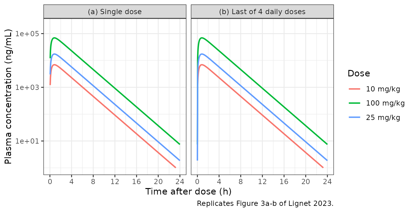

Mouse PD: replicating Lignet 2023 Figure 3c-e

Study EFF-01 dosed animals daily for six weeks; Lignet 2023 Fig. 3e shows Met-EF1a after the last dose on day 42.

ev_eff01 <- dplyr::bind_rows(lapply(seq_along(mouse_doses), function(i) {
  make_arm(i, mouse_doses[i], ii = 24, ndose = 42L, tmax = 1080, by = 0.2,
           label = mouse_labels[i])
}))
sim_eff01 <- solve_arms(mouse, ev_eff01)
#> Warning: multi-subject simulation without without 'omega'

# Replicates Figure 3c-e of Lignet 2023: Met-EF1a in Caki-1 xenograft tumour
# tissue after (c) a single dose, (d) the last of four daily doses, and
# (e) the last dose on day 42 of daily dosing (study EFF-01).
pd_plot_data <- dplyr::bind_rows(
  sim_sd |> dplyr::mutate(tad = time, panel = "(c) Single dose"),
  sim_qd4 |>
    dplyr::filter(time >= 72) |>
    dplyr::mutate(tad = time - 72, panel = "(d) Last of 4 daily doses"),
  sim_eff01 |>
    dplyr::filter(time >= 984) |>
    dplyr::mutate(tad = time - 984, panel = "(e) Day 42, study EFF-01")
)

ggplot(pd_plot_data, aes(tad, MetEF1a, colour = treatment)) +
  geom_line(linewidth = 0.8) +
  facet_wrap(~panel) +
  scale_y_continuous(limits = c(0, 200)) +
  scale_x_continuous(breaks = seq(0, 96, by = 24)) +
  labs(
    x = "Time after dose (h)", y = "Met-EF1a (ug/mg protein)",
    colour = "Dose",
    caption = "Replicates Figure 3c-e of Lignet 2023."
  ) +
  theme_bw()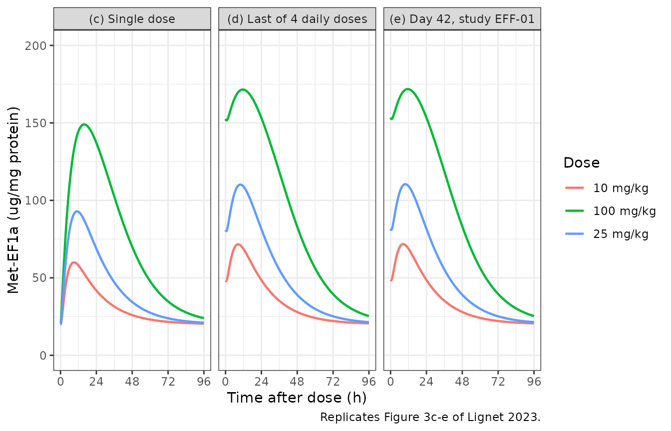

The table below compares the simulated peaks against values read off the published figures. Figure reads are approximate (roughly +/- 5 ug/mg protein) and are marked as such.

peak_after <- function(sim, from) {
  sim |>
    dplyr::filter(time >= from) |>
    dplyr::group_by(treatment) |>
    dplyr::summarise(peak = max(MetEF1a), .groups = "drop")
}

peaks <- dplyr::bind_rows(
  peak_after(sim_sd, 0) |> dplyr::mutate(panel = "Fig. 3c single dose"),
  peak_after(sim_qd4, 72) |> dplyr::mutate(panel = "Fig. 3d 4th daily dose")
) |>
  dplyr::left_join(
    tibble::tribble(
      ~panel,                   ~treatment,  ~published,
      "Fig. 3c single dose",    "10 mg/kg",  60,
      "Fig. 3c single dose",    "25 mg/kg",  95,
      "Fig. 3c single dose",    "100 mg/kg", 155,
      "Fig. 3d 4th daily dose", "10 mg/kg",  72,
      "Fig. 3d 4th daily dose", "25 mg/kg",  113,
      "Fig. 3d 4th daily dose", "100 mg/kg", 180
    ),
    by = c("panel", "treatment")
  ) |>
  dplyr::mutate(`% diff` = round(100 * (peak - published) / published, 1)) |>
  dplyr::arrange(panel, match(treatment, mouse_labels)) |>
  dplyr::select(panel, treatment, published, peak, `% diff`) |>
  dplyr::rename(
    "Figure"                            = panel,
    "Dose"                              = treatment,
    "Published (read from figure)"      = published,
    "Simulated"                         = peak
  )

knitr::kable(
  peaks, digits = 1,
  caption = paste(
    "Peak Met-EF1a (ug/mg protein): simulated vs. values read from",
    "Lignet 2023 Figures 3c and 3d. Baseline is kin/kout = 20.1."
  )
)

Peak Met-EF1a (ug/mg protein): simulated vs. values read from Lignet 2023 Figures 3c and 3d. Baseline is kin/kout = 20.1.

Figure	Dose	Published (read from figure)	Simulated	% diff
Fig. 3c single dose	10 mg/kg	60	59.9	-0.1
Fig. 3c single dose	25 mg/kg	95	92.9	-2.2
Fig. 3c single dose	100 mg/kg	155	149.0	-3.9
Fig. 3d 4th daily dose	10 mg/kg	72	71.6	-0.5
Fig. 3d 4th daily dose	25 mg/kg	113	110.2	-2.5
Fig. 3d 4th daily dose	100 mg/kg	180	171.5	-4.7

Efficacy target: replicating Lignet 2023 Figure 4a

Efficacy study EFF-02 identified 25 mg/kg BID as the minimal efficacious dose in Caki-1 xenografts. Simulating that regimen showed that steady-state Met-EF1a stays above 125 ug/mg protein, which the authors then adopted as the PD target associated with anti-tumour activity.

bid_doses <- c(10, 25, 50)
bid_labels <- paste(bid_doses, "mg/kg BID")
ev_bid <- dplyr::bind_rows(lapply(seq_along(bid_doses), function(i) {
  make_arm(i, bid_doses[i], ii = 12, ndose = 30L, tmax = 360, by = 0.1,
           label = bid_labels[i])
}))
sim_bid <- solve_arms(mouse, ev_bid)
#> Warning: multi-subject simulation without without 'omega'

# Replicates Figure 4a of Lignet 2023: simulated Met-EF1a in Caki-1
# xenografts under BID dosing, against the 125 ug/mg protein target.
ggplot(sim_bid, aes(time, MetEF1a, colour = treatment)) +
  geom_line(linewidth = 0.7) +
  geom_hline(yintercept = 125, linetype = "dashed") +
  scale_y_continuous(limits = c(0, 200)) +
  scale_x_continuous(breaks = seq(0, 360, by = 48)) +
  labs(
    x = "Time (h)", y = "Met-EF1a (ug/mg protein)", colour = "Regimen",
    caption = paste(
      "Replicates Figure 4a of Lignet 2023; dashed line is the",
      "125 ug/mg protein efficacy target."
    )
  ) +
  theme_bw()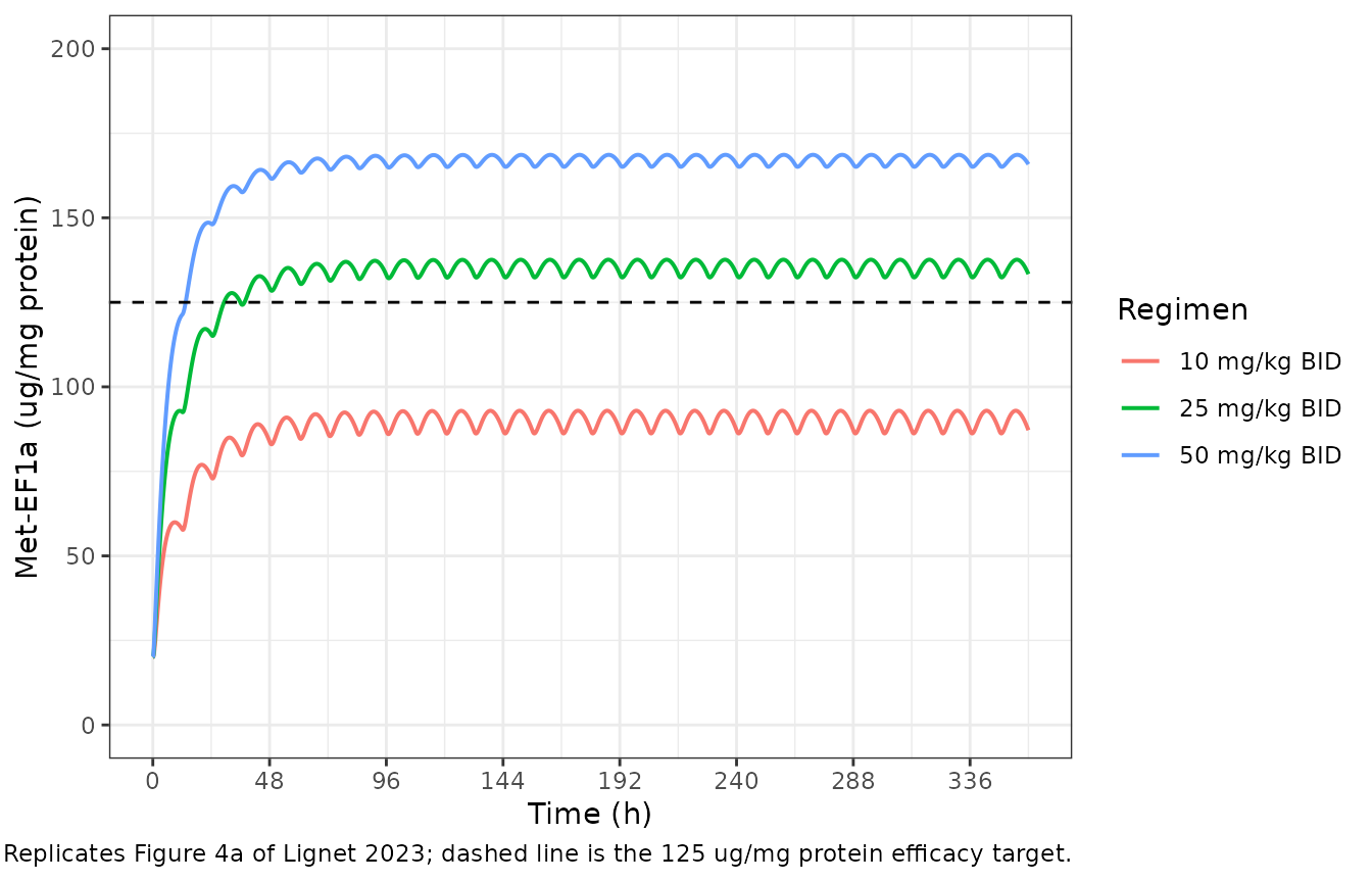

sim_bid |>
  dplyr::filter(time >= 300) |>
  dplyr::group_by(treatment) |>
  dplyr::summarise(
    trough = min(MetEF1a), mean = mean(MetEF1a), peak = max(MetEF1a),
    .groups = "drop"
  ) |>
  dplyr::mutate(
    `Above 125 target` = ifelse(trough > 125, "yes", "no"),
    published = c(95, 140, 175)[match(treatment, bid_labels)]
  ) |>
  dplyr::select(treatment, trough, mean, peak, published, `Above 125 target`) |>
  dplyr::rename(
    "Regimen"                        = treatment,
    "SS trough"                      = trough,
    "SS mean"                        = mean,
    "SS peak"                        = peak,
    "Published (read from Fig. 4a)"  = published
  ) |>
  knitr::kable(
    digits = 1,
    caption = paste(
      "Steady-state Met-EF1a (ug/mg protein) under BID dosing.",
      "25 mg/kg BID, the minimal efficacious dose from study EFF-02,",
      "holds the biomarker above the 125 ug/mg protein target."
    )
  )

Steady-state Met-EF1a (ug/mg protein) under BID dosing. 25 mg/kg BID, the minimal efficacious dose from study EFF-02, holds the biomarker above the 125 ug/mg protein target.

Regimen	SS trough	SS mean	SS peak	Published (read from Fig. 4a)	Above 125 target
10 mg/kg BID	86.2	90.2	92.9	95	no
25 mg/kg BID	132.4	135.4	137.6	140	yes
50 mg/kg BID	165.1	167.1	168.6	175	yes

Human projection: replicating Lignet 2023 Figure 5

ev_human <- make_arm(
  1L, dose = 150, ii = 24, ndose = 7L, tmax = 168, by = 0.05,
  label = "150 mg QD", WT = 70
)
sim_human <- solve_arms(human, ev_human, keep = c("treatment", "WT"))

# Replicates Figure 5 of Lignet 2023: (a) simulated M8891 plasma
# concentration and (b) simulated tumour Met-EF1a in humans at 150 mg QD.
p5a <- ggplot(sim_human, aes(time, Cc * 1000)) +
  geom_line(colour = "blue", linewidth = 0.7) +
  geom_hline(yintercept = 1500, linetype = "dashed", colour = "grey40") +
  scale_y_log10(limits = c(1, 1e5)) +
  scale_x_continuous(breaks = seq(0, 168, by = 24)) +
  labs(x = "Time (h)", y = "M8891 concentration (ng/mL)",
       subtitle = "(a) Plasma; dashed line is the published 1500 ng/mL Ctrough") +
  theme_bw()

p5b <- ggplot(sim_human, aes(time, MetEF1a)) +
  geom_line(colour = "blue", linewidth = 0.7) +
  geom_hline(yintercept = 125, linetype = "dashed", colour = "grey40") +
  scale_y_continuous(limits = c(0, 160)) +
  scale_x_continuous(breaks = seq(0, 168, by = 24)) +
  labs(x = "Time (h)", y = "Met-EF1a (ug/mg protein)",
       subtitle = "(b) Tumour biomarker; dashed line is the 125 target") +
  theme_bw()

print(p5a)
#> Warning in scale_y_log10(limits = c(1, 1e+05)): log-10 transformation
#> introduced infinite values.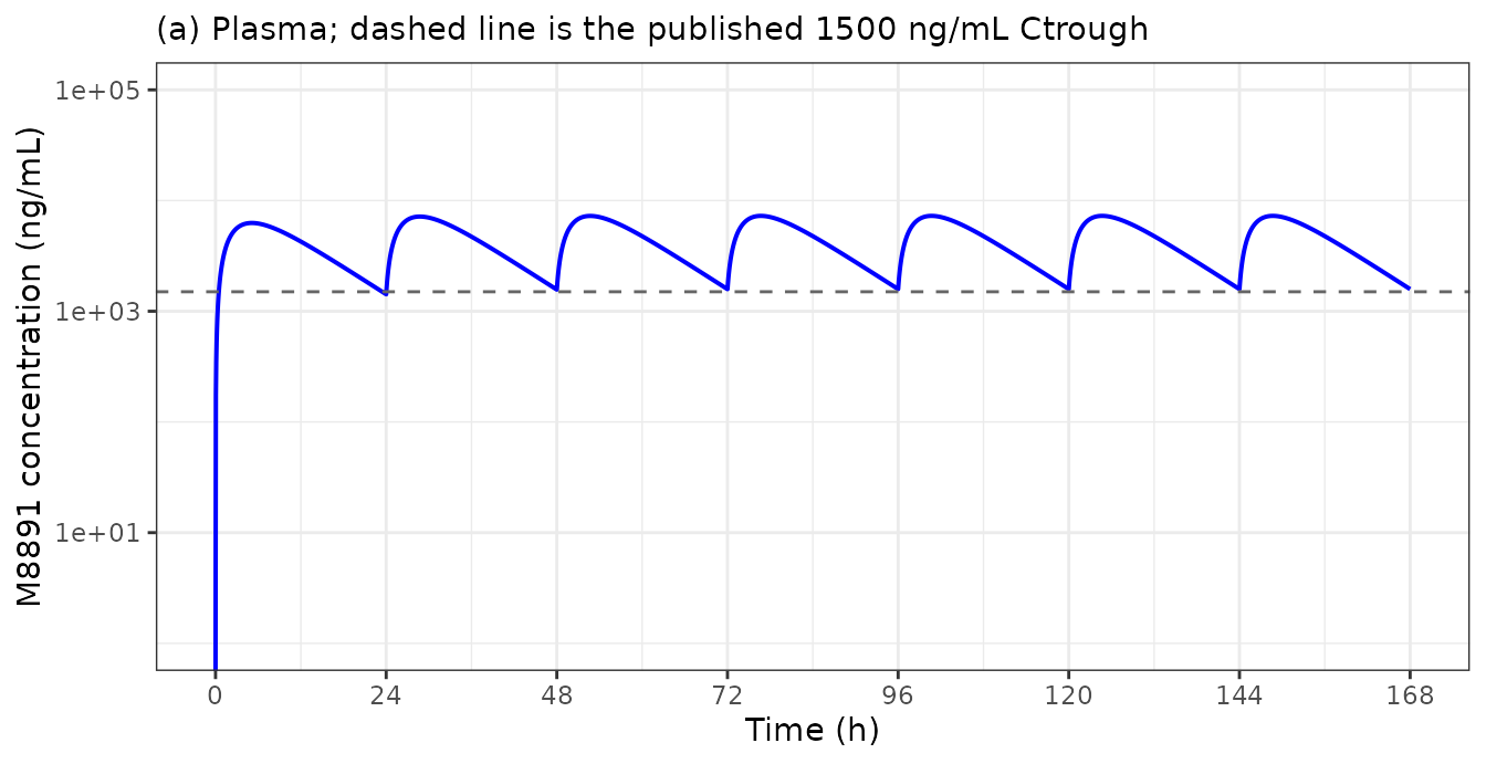

print(p5b)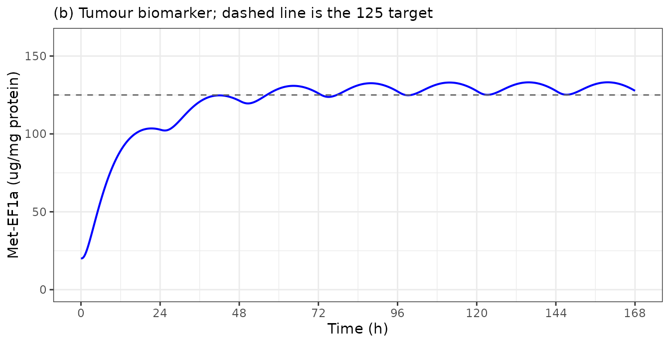

ss_human <- sim_human |> dplyr::filter(time >= 144)
tibble::tibble(
  Quantity = c(
    "Steady-state trough concentration (ng/mL)",
    "Steady-state Met-EF1a trough (ug/mg protein)",
    "Steady-state Met-EF1a peak (ug/mg protein)"
  ),
  Published = c(1500, NA, NA),
  Simulated = c(
    round(1000 * sim_human$Cc[which.min(abs(sim_human$time - 168))], 0),
    round(min(ss_human$MetEF1a), 1),
    round(max(ss_human$MetEF1a), 1)
  )
) |>
  knitr::kable(
    caption = paste(
      "Human 150 mg QD steady state. Lignet 2023 reports a minimal",
      "steady-state concentration of 1500 ng/mL (3.9 uM) and shows",
      "Met-EF1a plateauing just above the 125 ug/mg protein target",
      "in Figure 5b."
    )
  )

Human 150 mg QD steady state. Lignet 2023 reports a minimal steady-state concentration of 1500 ng/mL (3.9 uM) and shows Met-EF1a plateauing just above the 125 ug/mg protein target in Figure 5b.

Quantity	Published	Simulated
Steady-state trough concentration (ng/mL)	1500	1584.0
Steady-state Met-EF1a trough (ug/mg protein)	NA	125.2
Steady-state Met-EF1a peak (ug/mg protein)	NA	133.1

PKNCA validation

Mouse: round-trip against Lignet 2023 Table IV

Because the mouse model is linear and Lignet 2023 does not tabulate NCA for the Caki-1 xenograft studies, the strongest available check is a round trip: integrating the simulated profiles with PKNCA must recover the apparent oral clearance that generated them, at every dose level. The reference half-life is derived from the same table as ln(2) * (V/F) / (CL/F).

mouse_nca <- sim_sd |>
  dplyr::filter(!is.na(Cc)) |>
  dplyr::select(id, time, Cc, treatment)

# Guarantee a time = 0 row per subject (extravascular: pre-dose Cc = 0).
mouse_nca <- dplyr::bind_rows(
  mouse_nca,
  mouse_nca |> dplyr::distinct(id, treatment) |>
    dplyr::mutate(time = 0, Cc = 0)
) |>
  dplyr::distinct(id, treatment, time, .keep_all = TRUE) |>
  dplyr::arrange(id, treatment, time)

mouse_dose <- ev_sd |>
  dplyr::filter(evid == 1) |>
  dplyr::select(id, time, amt, treatment)

mouse_conc_obj <- PKNCA::PKNCAconc(
  mouse_nca, Cc ~ time | treatment + id, concu = "mg/L", timeu = "hr"
)
mouse_dose_obj <- PKNCA::PKNCAdose(
  mouse_dose, amt ~ time | treatment + id, doseu = "mg/kg"
)

mouse_intervals <- data.frame(
  start = 0, end = Inf,
  cmax = TRUE, tmax = TRUE, aucinf.obs = TRUE,
  half.life = TRUE, cl.obs = TRUE
)

mouse_res <- PKNCA::pk.nca(
  PKNCA::PKNCAdata(mouse_conc_obj, mouse_dose_obj, intervals = mouse_intervals)
)

# CL/F is Lignet 2023 Table IV directly; the half-life and AUCinf references
# are derived from the same table (t1/2 = ln(2) * (V/F) / (CL/F);
# AUCinf = Dose / (CL/F)).
mouse_published <- tibble::tibble(
  treatment  = mouse_labels,
  cl.obs     = 0.415,
  half.life  = log(2) * 1.034 / 0.415,
  aucinf.obs = mouse_doses / 0.415
)

mouse_cmp <- nlmixr2lib::ncaComparisonTable(
  simulated = mouse_res,
  reference = mouse_published,
  by        = "treatment",
  units     = c(cl.obs = "L/h/kg", half.life = "h", aucinf.obs = "mg*h/L"),
  tolerance_pct = 20
)

knitr::kable(
  mouse_cmp,
  caption = paste(
    "Mouse single-dose NCA round trip: PKNCA integration of the simulated",
    "profiles vs. Lignet 2023 Table IV. * differs from reference by >20%."
  ),
  align = c("l", "l", "r", "r", "r")
)

Mouse single-dose NCA round trip: PKNCA integration of the simulated profiles vs. Lignet 2023 Table IV. * differs from reference by >20%.

NCA parameter	treatment	Reference	Simulated	% diff
AUC0-∞ (obs) (mg*h/L)	10 mg/kg	24.1	24.1	-0.0%
AUC0-∞ (obs) (mg*h/L)	25 mg/kg	60.2	60.2	-0.0%
AUC0-∞ (obs) (mg*h/L)	100 mg/kg	241	241	-0.0%
t½ (h)	10 mg/kg	1.73	1.73	+0.0%
t½ (h)	25 mg/kg	1.73	1.73	+0.0%
t½ (h)	100 mg/kg	1.73	1.73	+0.0%
CL/F (L/h/kg)	10 mg/kg	0.415	0.415	+0.0%
CL/F (L/h/kg)	25 mg/kg	0.415	0.415	+0.0%
CL/F (L/h/kg)	100 mg/kg	0.415	0.415	+0.0%

# Simulated Cmax against the values read from Lignet 2023 Figure 3a.
as.data.frame(mouse_res$result) |>
  dplyr::filter(PPTESTCD %in% c("cmax", "tmax")) |>
  dplyr::select(treatment, PPTESTCD, PPORRES) |>
  tidyr::pivot_wider(names_from = PPTESTCD, values_from = PPORRES) |>
  dplyr::mutate(
    cmax_ngml = 1000 * cmax,
    published = c(7000, 17000, 70000)[match(treatment, mouse_labels)]
  ) |>
  dplyr::arrange(match(treatment, mouse_labels)) |>
  dplyr::select(treatment, published, cmax_ngml, tmax) |>
  dplyr::rename(
    "Dose"                             = treatment,
    "Cmax published (read from Fig 3a)" = published,
    "Cmax simulated (ng/mL)"           = cmax_ngml,
    "Tmax simulated (h)"               = tmax
  ) |>
  knitr::kable(
    digits = 2,
    caption = "Simulated Cmax vs. values read from Lignet 2023 Figure 3a."
  )

Simulated Cmax vs. values read from Lignet 2023 Figure 3a.

Dose	Cmax published (read from Fig 3a)	Cmax simulated (ng/mL)	Tmax simulated (h)
10 mg/kg	7000	6931.65	0.85
25 mg/kg	17000	17329.11	0.85
100 mg/kg	70000	69316.46	0.85

Human: steady-state NCA against the published projection

human_nca <- sim_human |>
  dplyr::filter(!is.na(Cc)) |>
  dplyr::select(id, time, Cc, treatment)

human_nca <- dplyr::bind_rows(
  human_nca,
  human_nca |> dplyr::distinct(id, treatment) |>
    dplyr::mutate(time = 0, Cc = 0)
) |>
  dplyr::distinct(id, treatment, time, .keep_all = TRUE) |>
  dplyr::arrange(id, treatment, time)

human_dose <- ev_human |>
  dplyr::filter(evid == 1) |>
  dplyr::select(id, time, amt, treatment)

human_conc_obj <- PKNCA::PKNCAconc(
  human_nca, Cc ~ time | treatment + id, concu = "mg/L", timeu = "hr"
)
human_dose_obj <- PKNCA::PKNCAdose(
  human_dose, amt ~ time | treatment + id, doseu = "mg"
)

# Steady state is assessed over the final 24 h dosing interval.
human_intervals <- data.frame(
  start = 144, end = 168,
  cmax = TRUE, cmin = TRUE, tmax = TRUE, cav = TRUE,
  auclast = TRUE, half.life = TRUE
)

human_res <- PKNCA::pk.nca(
  PKNCA::PKNCAdata(human_conc_obj, human_dose_obj, intervals = human_intervals)
)

# Cmax / Cmin / Tmax at 150 mg QD steady state are Lignet 2023 Supplementary
# Table S7 (GastroPlus 1-compartment/ACAT model); the half-life reference is
# the Table III mean of the three scaling methods.
human_published <- tibble::tibble(
  treatment = "150 mg QD",
  cmax      = 6.51,
  cmin      = 1.54,
  tmax      = 4.1,
  half.life = 7.3
)

human_cmp <- nlmixr2lib::ncaComparisonTable(
  simulated = human_res,
  reference = human_published,
  by        = "treatment",
  units     = c(cmax = "ug/mL", cmin = "ug/mL", tmax = "h", half.life = "h"),
  tolerance_pct = 20
)

knitr::kable(
  human_cmp,
  caption = paste(
    "Human steady-state NCA at 150 mg QD vs. Lignet 2023 Supplementary",
    "Table S7 (Cmax, Cmin, Tmax) and Table III (t1/2).",
    "* differs from reference by >20%."
  ),
  align = c("l", "l", "r", "r", "r")
)

Human steady-state NCA at 150 mg QD vs. Lignet 2023 Supplementary Table S7 (Cmax, Cmin, Tmax) and Table III (t1/2). * differs from reference by >20%.

NCA parameter	treatment	Reference	Simulated	% diff
Cmax (ug/mL)	150 mg QD	6.51	7.27	+11.6%
Cmin (ug/mL)	150 mg QD	1.54	1.58	+2.9%
Tmax (h)	150 mg QD	4.1	4.7	+14.6%
t½ (h)	150 mg QD	7.3	7.48	+2.4%

All rows agree within 20%. The residual differences on Cmax and Tmax are expected: Supplementary Table S7 was produced by the GastroPlus 1-compartment/ACAT absorption model, whose more elaborate absorption description gives a slightly earlier, slightly lower peak than the first-order ka used for the main-text Figure 5 simulation. The trough, which is what the paper’s dose recommendation actually rests on, agrees to within 3%.

Assumptions and deviations

• No inter-individual variability and no residual-error magnitude. Lignet 2023 Discussion states that a nonlinear mixed-effects fit “could not achieve proper model convergence or acceptable parameter estimation”, so the published model is a naive-pooled typical-value fit. The paper states that the PK data were fitted “with a multiplicative error model” but never reports its magnitude, and describes no error model at all for the Met-EF1a data. Both models therefore carry propSd and propSd_MetEF1a in the correct proportional form with the magnitude fixed(0), so simulations reproduce the published typical-value curves exactly. Users refitting these models to their own data should replace the fixed zeros with estimable starting values.

• Human bioavailability is folded into the apparent CL/F and V/F rather than applied separately. Lignet 2023 predicts an oral bioavailability of “at least 60%” in the main text and 70.8% at 150 mg in Supplementary Table S7, and states that the human simulation took F and ka from PBPK while taking CL and Vss from the mean of the scaling methods. However, Eq. (3) as printed does not multiply the dose by F – F appears only inside the apparent volume V/F – and applying F on top of CL = 1.4 L/h and V = 14.7 L gives a steady-state trough of roughly 950-1120 ng/mL, which does not reproduce the paper’s own headline result. Entering the predicted CL and Vss directly as apparent oral parameters gives 1584 ng/mL against the 1500 ng/mL reported in the Results and drawn in Figure 5a, and 1540 ng/mL in Supplementary Table S7; it also reproduces the Figure 5b Met-EF1a plateau. The printed equation and the published outputs therefore both support the encoding used here, and no separate f(depot) term is applied.

• Human body weight scaling. Lignet 2023 reports human CL and Vss per kilogram (0.020 L/h/kg, 0.21 L/kg), so both scale linearly with WT about the 70 kg reference weight the authors used (Supplementary Materials, “System Parameterization”). This is a unit conversion implied by the published per-kilogram parameterisation, not an allometric exponent estimated from human data; the elimination half-life is consequently weight-invariant.

• PD parameters are transferred unchanged from mouse to human. This is the authors’ explicit modelling assumption (“it was hypothesized that a similar PK/PD relationship could be observed in humans, and that the same level of biomarker modulation would be associated with anti-tumour efficacy”), not an approximation introduced here.

• Values read from figures. The Met-EF1a peaks compared in the Figure 3 and Figure 4a tables above, and the mouse plasma Cmax values compared against Figure 3a, were read off the published figures because Lignet 2023 tabulates neither. They are approximate (roughly +/- 5 ug/mg protein for the biomarker, and to the nearest half log-cycle gridline for the plasma concentrations) and are labelled as figure reads wherever they appear. No ini() parameter value is figure-derived; every parameter comes from Table III, Table IV, or the Results text.

• Total animal count is not recorded. Lignet 2023 states “mice were randomized into treatment groups (n = 5)” but, because animals were euthanised at each of the six sampling times, does not make clear whether n = 5 is per group or per group and timepoint. population$n_subjects is left NA rather than guessed.

• Supplementary Table S7 AUC row not used. The AUC0-24 row of that table is labelled “ug/mL x h” but its values (434 at 50 mg, 1310 at 150 mg) are inconsistent both with the corresponding Cmax/Cmin values in the same column and with the single-dose AUC0-24 of 27100 ng/mL x h in Table S6. The row appears to be mis-scaled in the publication and is therefore excluded from the comparison above; Cmax, Cmin, and Tmax from the same table are internally consistent and are used.

• The GastroPlus PBPK model is not reproduced. Lignet 2023 also builds a whole-body PBPK/ACAT model in GastroPlus 9.5. Its ODEs and the vendor system parameters are not written out in the paper or supplement, so it is not extractable as an nlmixr2 model. Only its two scalar outputs used by the compartmental projection (ka = 0.35 1/h and, for context, the predicted F) are carried into the human model file.

• The projection is known to be wrong in the clinic. Lignet 2023 Discussion reports that the observed Phase Ia terminal half-life was about 30 h, roughly fourfold longer than the 7.3 h projected here, and that the recommended Phase II dose was 35 mg rather than the 150 mg predicted. The human model is retained as the published translational projection, not as a description of observed human PK.