Fazpilodemab (Yoshida 2024)
Source:vignettes/articles/Yoshida_2024_fazpilodemab.Rmd
Yoshida_2024_fazpilodemab.RmdModel and source
- Citation: Yoshida K, Poon V, Dash A, Kunder R, Chinn L, Kagedal M. Simulation-based evaluation of personalized dosing approaches for anti-FGFR/KLB bispecific antibody fazpilodemab. CPT Pharmacometrics Syst Pharmacol. 2024;13(4):544-550. doi:10.1002/psp4.13111
- Description: Population PK + longitudinal gastrointestinal-adverse-event (GIAE) discrete-time Markov + treatment-discontinuation logistic model for the anti-FGFR/KLB bispecific antibody fazpilodemab (BFKB8488A) in adults with type 2 diabetes mellitus or non-alcoholic fatty liver disease (Yoshida 2024). The PK structure is a 2-compartment disposition with parallel direct (ka) plus transit-mediated (ka2 via the depot2 absorption compartment, transit rate ktr) subcutaneous absorption; linear plus Michaelis-Menten elimination acting on free drug; target-mediated quasi-steady-state binding to a constant target concentration rmax; and a sigmoidal time-onset ADA-mediated clearance arm cl_ada that activates when ADA_POS = 1. The DTMM transition probabilities (grade 0 / grade 1 / grade 2-3) and the treatment-discontinuation probability are emitted as algebraic outputs conditional on the time-varying PREV_AE_SCORE covariate (the previous-day GIAE grade); the actual Markov-chain stochastic simulation is performed downstream in R using these probabilities (matching the mrgsolve plus Rcpp framework of the source paper supplement S2.3).
- Article: https://doi.org/10.1002/psp4.13111
- Supplement (figures): bundled with article DOI
- Supplement (model code, Text S1 + S2): bundled with article DOI; contains the NONMEM control stream for the longitudinal AE model and the full mrgsolve typical-value listing used for the dynamic clinical-trial simulations
Population
Yoshida 2024 used data from the multiple-ascending-dose study GC39547 (NCT03060538) of fazpilodemab (BFKB8488A) in patients with type 2 diabetes mellitus (T2DM) and non-alcoholic fatty liver disease (NAFLD). 121 patients received fazpilodemab and 32 received placebo (n = 153 total). Fazpilodemab was administered subcutaneously in the abdomen or thigh at 10-250 mg with q1w, q2w, or q4w intervals. Detailed demographics (age / weight / sex / race) are not reported in the main text or in the supplements bundled with this article; the text extracted from Supplements 1 (figures) and 2 (model code) contains neither a Table 1 baseline-demographics summary nor an extended-text demographics paragraph.
The population PK model was characterised as “unpublished data” in
the main text (Methods page 545), but the typical-value parameter set
with IIV / IOV / residual error is given in full as the mrgsolve
[PARAM] / [OMEGA] / [SIGMA] block
of Supplement S2.3.1.
readModelDb("Yoshida_2024_fazpilodemab")()$population
#> $species
#> [1] "human"
#>
#> $n_subjects
#> [1] 153
#>
#> $n_studies
#> [1] 1
#>
#> $age_range
#> [1] "Adults (specific age range not reported in main text or available supplement)"
#>
#> $weight_range
#> [1] "Adults (specific weight range not reported in main text or available supplement)"
#>
#> $sex_female_pct
#> [1] NA
#>
#> $race_ethnicity
#> [1] "Not reported in main text or available supplement"
#>
#> $disease_state
#> [1] "Type 2 diabetes mellitus (T2DM) or non-alcoholic fatty liver disease (NAFLD)"
#>
#> $dose_range
#> [1] "10-250 mg subcutaneous q1w, q2w, or q4w"
#>
#> $regions
#> [1] "Not reported in main text or available supplement"
#>
#> $notes
#> [1] "Multiple ascending dose (MAD) study GC39547 (NCT03060538). 121 patients with T2DM or NAFLD received fazpilodemab and 32 patients received placebo (n = 153 total). Fazpilodemab was administered subcutaneously in the abdomen or thigh at 10-250 mg with intervals of q1w, q2w, or q4w. Detailed demographic breakdown (age / weight / sex / race) is not reported in the main text or in the available supplements; the available Supplements 1 (figures) and 2 (model code) contain neither a Table 1 baseline-demographics summary nor an extended-text demographics paragraph. Phase I/II population characterisation; full popPK described as 'unpublished data' in the main text, with the typical-value parameter set and IIV/IOV/residual error provided in full as the mrgsolve [PARAM] / [OMEGA] / [SIGMA] block of Supplement S2.3.1."
Source trace
The per-parameter origin is recorded as an in-file comment next to
each ini() entry in
inst/modeldb/specificDrugs/Yoshida_2024_fazpilodemab.R. All
typical values come from the mrgsolve [PARAM] block of
Supplement S2.3.1. The table below collects the audit trail in one
place. Concentration / volume / mass constants from the supplement
(units: ug, L, day) have been rescaled to the model’s mg / L / day /
(ug/mL) units; the conversion is 1 mg = 1000 ug, so VMAX, KM, RMAX, and
KSS are divided by 1000 (other constants are unit-invariant).
| Parameter / equation | Value in model | Source (Supplement S2.3.1 mrgsolve [PARAM]) |
|---|---|---|
lka |
log(0.243) | TVKA = 0.243 (1/day) |
lktr |
log(0.115) | TVKTR = 0.115 (1/day) |
lka2 |
log(0.0687) | TVKA2 = 0.0687 (1/day) |
lcl |
log(0.349) | TVCL = 0.349 (L/day) |
lvc |
log(2.98) | TVV2 = 2.98 (L) |
lvp |
log(1.83) | TVV3 = 1.83 (L) |
lq |
log(3.07) | TVQ = 3.07 (L/day) |
lvmax |
log(3.34) | TVVMAX = 3340 ug/day = 3.34 mg/day |
lkm |
log(0.482) | TVKM = 482 ug/L = 0.482 ug/mL |
lrmax |
fixed(log(2)) | TVRMAX = 2000 ug/L = 2 ug/mL (fixed, no target turnover) |
lkss |
log(0.0885) | TVKSS = 88.5 ug/L = 0.0885 ug/mL |
lfdepot |
log(0.719) | TVF1 = 0.719 |
lcl_ada |
log(3.39) | TVCLADAMAX = 3.39 (L/day) |
lt50_ada |
log(46.6) | TVT50ADA = 46.6 (day) |
lk_ada |
log(0.195) | TVKADA = 0.195 (1/day) |
lslp_ae |
log(0.0927) | TVSLP = 0.0927 per (ug/mL); matches main-text “9.72% odds increase per ug/mL” = log(1.0972) |
b1_g0_ae |
-4.69 | TV0B1 = -4.69 |
b2b1_g0_ae |
-0.799 | TV0B2B1 = -0.799 |
b1_g1_ae |
2.4 | TV1B1 = 2.4 |
b2b1_g1_ae |
-14.8 | TV1B2B1 = -14.8 |
b1_g2_ae |
1.83 | TV2B1 = 1.83 |
b2b1_g2_ae |
-0.037 | TV2B2B1 = -0.037 |
tef_g0_ae |
-0.0336 | TIME_EFF = -0.0336 |
b_dc_g0 |
-4.31 | B_discon_G0 = -4.31 |
b_dc_g1 |
-1.69 | B_discon_G1 = -1.69 (= -4.31 + 2.62) |
b_dc_g2 |
-1.33 | B_discon_G2 = -1.33 (= -4.31 + 2.98) |
etalcl |
0.0174 (var) | E_CL = 0.0174 |
etalfdepot |
0.0952 (var) | E_F1 = 0.0952 |
etalvc |
0.286 (var) | E_V2 = 0.286 |
etalka2 |
0.297 (var) | E_KA2 = 0.297 |
etalcl_ada |
5.21 (var) | E_CLADAMAX = 5.21 |
etalt50_ada |
0.155 (var) | E_T50ADA = 0.155 |
etalslp_ae |
1.85 (var) | E_SLP = 1.85 |
propSd |
sqrt(0.0437) | EPSP = 0.0437 (variance) -> SD ~ 0.209 |
d/dt(depot) |
-kadepot - ktrdepot | mrgsolve [ODE] dxdt_A1 = -KAA1 - KTRA1 |
d/dt(depot2) |
ktrdepot - ka2depot2 | mrgsolve [ODE] dxdt_A4 = KTRA1 - KA2A4 |
d/dt(central) |
kadepot + ka2depot2 + qperipheral1/vp - (cl + cl_ada + q)cfree - vmax*cfree/(km + cfree) | mrgsolve [ODE] dxdt_A2 |
d/dt(peripheral1) |
q*(cfree - peripheral1/vp) | mrgsolve [ODE] dxdt_A3 = Q*(CFREE - A3/V3) |
cfree (QSS) |
0.5 * (disc + sqrt(disc^2 + 4kssctot)); disc = ctot - rmax - kss | mrgsolve [ODE] CFREE = 0.5(A2/V2 - RMAX - KSS) +
0.5sqrt((A2/V2 - RMAX - KSS)^2 + 4KSSA2/V2) (Gibiansky
2008 QSS with constant target) |
cl_ada (sigmoidal) |
ADA_POS * cl_ada_max / (1 + exp(-k_ada*(time - t50_ada))) | mrgsolve [ODE] CLADA =
ADA2CLADAMAX/(1+exp(-KADA(SOLVERTIME + TIMEinit -
T50ADA))) |
| DTMM transition logits | LGT1 = B1 + slp_ae * Cc; LGT2 = B2 + slp_ae * Cc; B1/B2 selected from PREV_AE_SCORE | mrgsolve [TABLE] LGT1/LGT2 = B1/B2 +
SLP*CFREE/1000 |
| Discontinuation logit | b_dc selected from PREV_AE_SCORE; p_dc = expit(b_dc) | mrgsolve [TABLE] LGTdiscon = G0*B_discon_G0 + …;
Pdiscon = expit(LGTdiscon) |
Virtual cohort
Original observed data are not publicly available. We build virtual cohorts that match the four q2w dose levels from the phase II dose-selection analysis (Figure 2a of the source paper: 50, 75, 100, 130 mg q2w; Methods page 545 mentions the phase II dose set 50 / 75 / 100 mg q2w used in study GC41033).
set.seed(20240101)

n_per_arm <- 30L   # small VPC; multi-eta simulation across 4 arms is expensive
dose_levels <- c(50, 75, 100, 130)
sim_duration_days <- 84L   # 12 weeks (paper's exposure window for AUCss / Cmax,ss)
n_doses <- ceiling(sim_duration_days / 14) + 1L

make_cohort <- function(n, amt_mg, id_offset, ada_frac = 0.0) {
  doses <- rxode2::et(amt = amt_mg, cmt = "depot", ii = 14, addl = n_doses - 1L)
  ev <- rxode2::et(doses, seq(0, sim_duration_days, by = 2), cmt = "central")
  ev <- as.data.frame(ev)
  ev_list <- lapply(seq_len(n), function(i) {
    out <- ev
    out$id <- id_offset + i
    out$ADA_POS <- rbinom(1L, 1L, ada_frac)
    out$PREV_AE_SCORE <- 0L
    out$dose_mg <- amt_mg
    out
  })
  dplyr::bind_rows(ev_list)
}

events <- bind_rows(
  make_cohort( n_per_arm,  50, id_offset =   0L),
  make_cohort( n_per_arm,  75, id_offset = 100L),
  make_cohort( n_per_arm, 100, id_offset = 200L),
  make_cohort( n_per_arm, 130, id_offset = 300L)
)

stopifnot(!anyDuplicated(unique(events[, c("id", "time", "evid")])))
nrow(events)
#> [1] 5280
table(events$dose_mg[events$evid == 1L]) / n_doses
#>
#>       50       75      100      130
#> 4.285714 4.285714 4.285714 4.285714
Simulation
mod <- readModelDb("Yoshida_2024_fazpilodemab")
sim <- rxode2::rxSolve(mod, events = events, keep = c("dose_mg", "ADA_POS")) |>
  as.data.frame()
#> ℹ parameter labels from comments will be replaced by 'label()'
Replicate published figures
Figure 2a (dose vs concentration profile)
Figure 2a of the source paper shows simulated dose-vs-response
relationships for liver fat reduction and persistent GIAE; the
underlying PK exposure that feeds those relationships is the
steady-state plasma profile produced by the popPK model. The
exposure-response transformations (sigmoidal Emax for liver fat;
logistic regression for persistent GIAE) are not numerically
parameterized anywhere in the source paper or its supplement (the
supplement S2.1 R script fits them via
rstanemax::stan_emax() and stats::glm() but
does not list the fitted point estimates), so they are NOT encoded in
this model file. The exposure simulation that those E-R models would
consume is shown below.
sim |>
  group_by(time, dose_mg) |>
  summarise(
    Q05 = quantile(Cc, 0.05),
    Q50 = quantile(Cc, 0.50),
    Q95 = quantile(Cc, 0.95),
    .groups = "drop"
  ) |>
  ggplot(aes(time, Q50, fill = factor(dose_mg))) +
  geom_ribbon(aes(ymin = Q05, ymax = Q95), alpha = 0.25) +
  geom_line(aes(color = factor(dose_mg))) +
  scale_y_log10() +
  labs(
    x = "Time (day)",
    y = "Free fazpilodemab Cc (ug/mL)",
    color = "Dose (mg q2w)",
    fill  = "Dose (mg q2w)",
    title = "Simulated steady-state PK profiles at four q2w dose levels",
    caption = "Replicates the exposure inputs underlying Figure 2a of Yoshida 2024."
  )
#> Warning in scale_y_log10(): log-10 transformation introduced infinite values.
#> log-10 transformation introduced infinite values.
#> log-10 transformation introduced infinite values.
#> log-10 transformation introduced infinite values.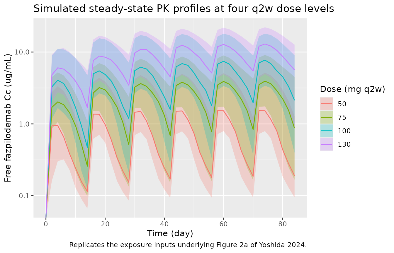
ADA-mediated clearance time course
The ADA-mediated clearance arm is a sigmoidal time-onset function
that activates when ADA_POS = 1. Below we show the time
course for typical-value subjects in the ADA-positive and ADA-negative
arms.
mod_typ <- mod |> rxode2::zeroRe()
#> ℹ parameter labels from comments will be replaced by 'label()'

ev_ada <- rxode2::et(amt = 100, cmt = "depot", ii = 14, addl = 11) |>
  rxode2::et(seq(0, 180, by = 2), cmt = "central")
ev_ada_pos <- ev_ada
ev_ada_pos$ADA_POS <- 1
ev_ada_pos$PREV_AE_SCORE <- 0
ev_ada_neg <- ev_ada
ev_ada_neg$ADA_POS <- 0
ev_ada_neg$PREV_AE_SCORE <- 0

sim_ada <- bind_rows(
  rxode2::rxSolve(mod_typ, ev_ada_pos) |> as.data.frame() |> mutate(ADA = "positive"),
  rxode2::rxSolve(mod_typ, ev_ada_neg) |> as.data.frame() |> mutate(ADA = "negative")
)
#> ℹ omega/sigma items treated as zero: 'etalcl', 'etalfdepot', 'etalvc', 'etalka2', 'etalcl_ada', 'etalt50_ada', 'etalslp_ae'
#> ℹ omega/sigma items treated as zero: 'etalcl', 'etalfdepot', 'etalvc', 'etalka2', 'etalcl_ada', 'etalt50_ada', 'etalslp_ae'

ggplot(sim_ada, aes(time, Cc, color = ADA)) +
  geom_line() +
  scale_y_log10() +
  labs(
    x = "Time (day)",
    y = "Free fazpilodemab Cc (ug/mL)",
    color = "ADA status",
    title = "Effect of ADA on fazpilodemab exposure (typical-value 100 mg q2w)",
    caption = paste(
      "Typical-value simulation (no IIV). ADA-mediated clearance ramps up",
      "sigmoidally with T50_ada = 46.6 days; ADA-positive subjects show a",
      "marked exposure decrease after the second month of dosing."
    )
  )
#> Warning in scale_y_log10(): log-10 transformation introduced infinite values.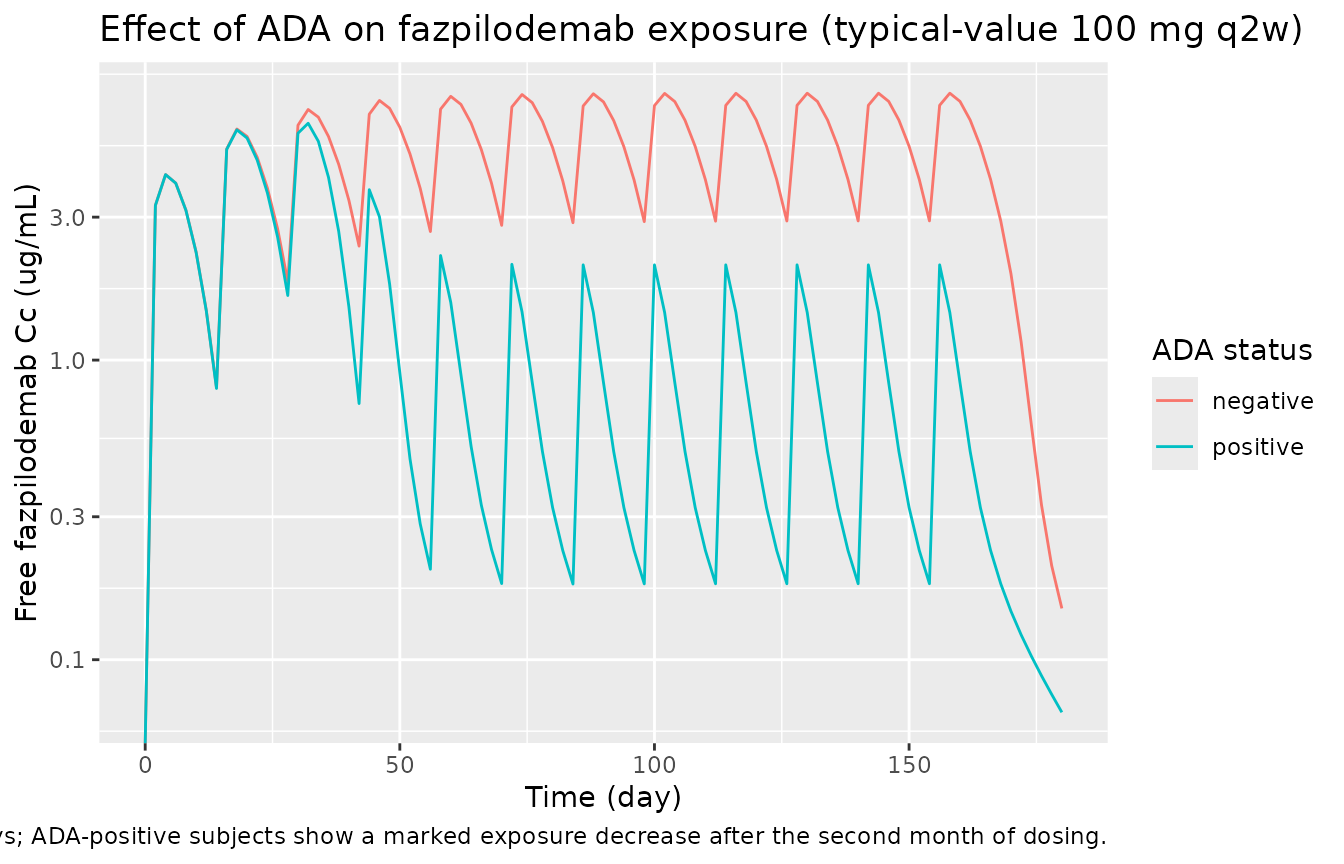
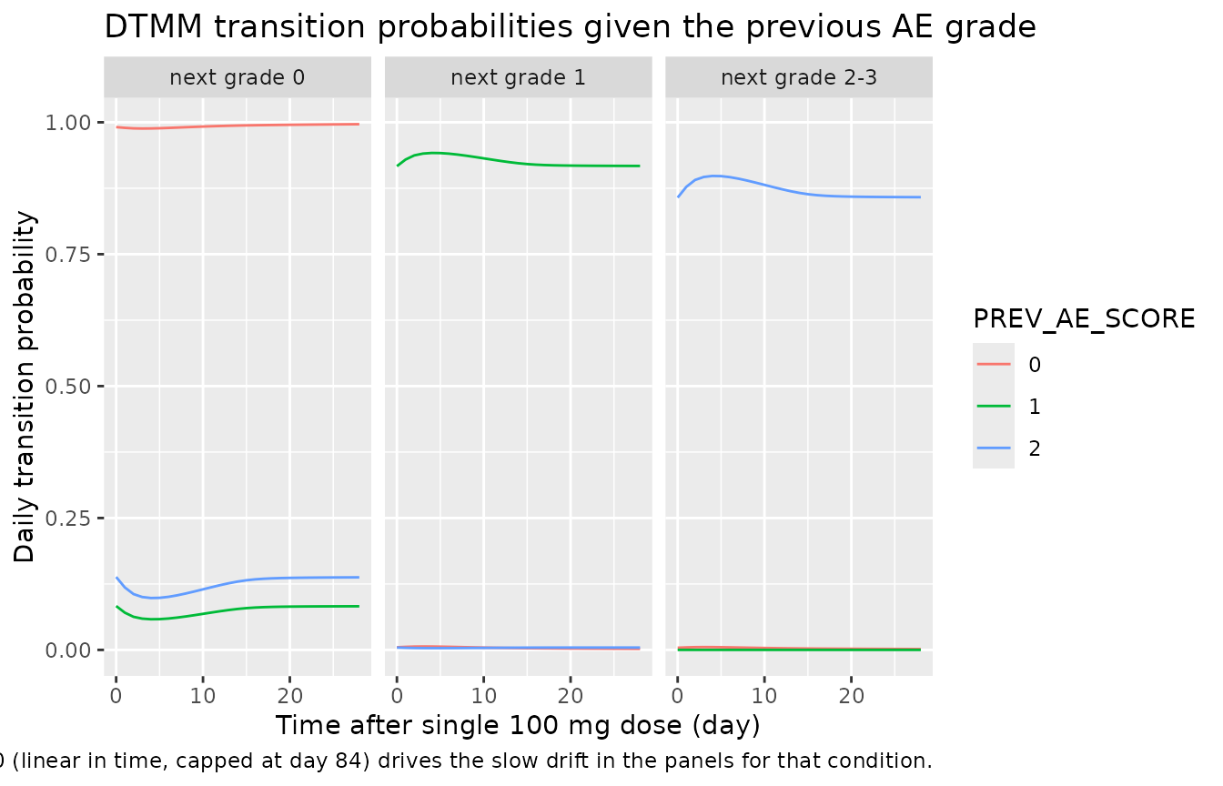
DTMM transition probabilities (algebraic outputs)
The longitudinal GIAE model is a daily discrete-time Markov model
with three states: grade 0, grade 1, and grade 2/3 (combined). At each
daily transition the probability of moving to each next state depends on
(i) the current state (via PREV_AE_SCORE), (ii) the current
free fazpilodemab concentration (via the slope lslp_ae),
and (iii) the time since first dose (via tef_g0_ae, applied
only when PREV_AE_SCORE = 0 and capped at day 84). The
actual stochastic state transitions are performed in R (or any host
language) using the algebraic transition probabilities emitted by this
model.
The chart below shows the transition probabilities at the time-of-peak concentration after a single 100 mg dose, as a function of the previous AE grade.
ev_dtmm <- rxode2::et(amt = 100, cmt = "depot") |>
  rxode2::et(seq(0, 28, by = 1), cmt = "central")
ev_dtmm$ADA_POS <- 0

dtmm_long <- bind_rows(lapply(0:2, function(prev) {
  evx <- ev_dtmm
  evx$PREV_AE_SCORE <- prev
  r <- rxode2::rxSolve(mod_typ, evx) |> as.data.frame()
  data.frame(
    time = r$time,
    Cc = r$Cc,
    prev_grade = prev,
    p_g0 = r$p_ae_g0,
    p_g1 = r$p_ae_g1,
    p_g23 = r$p_ae_g23,
    p_dc = r$p_dc
  )
}))
#> ℹ omega/sigma items treated as zero: 'etalcl', 'etalfdepot', 'etalvc', 'etalka2', 'etalcl_ada', 'etalt50_ada', 'etalslp_ae'
#> ℹ omega/sigma items treated as zero: 'etalcl', 'etalfdepot', 'etalvc', 'etalka2', 'etalcl_ada', 'etalt50_ada', 'etalslp_ae'
#> ℹ omega/sigma items treated as zero: 'etalcl', 'etalfdepot', 'etalvc', 'etalka2', 'etalcl_ada', 'etalt50_ada', 'etalslp_ae'

dtmm_long |>
  pivot_longer(c(p_g0, p_g1, p_g23), names_to = "next_state", values_to = "p") |>
  mutate(
    next_state = recode(next_state,
                        p_g0 = "next grade 0",
                        p_g1 = "next grade 1",
                        p_g23 = "next grade 2-3")
  ) |>
  ggplot(aes(time, p, color = factor(prev_grade))) +
  geom_line() +
  facet_wrap(~next_state) +
  labs(
    x = "Time after single 100 mg dose (day)",
    y = "Daily transition probability",
    color = "PREV_AE_SCORE",
    title = "DTMM transition probabilities given the previous AE grade",
    caption = paste(
      "From left: probability that the next-day grade is 0, 1, or 2/3,",
      "conditional on the previous grade. The time effect on B1 / B2 when",
      "PREV_AE_SCORE = 0 (linear in time, capped at day 84) drives the",
      "slow drift in the panels for that condition."
    )
  )
Discontinuation probability
The treatment-discontinuation model is a logistic regression on the
current GIAE grade; in the source paper’s mrgsolve simulation it is
evaluated once per 14-day dosing cycle and gated to
PREV_AE_SCORE > 0 (no discontinuation from grade 0). The
algebraic output p_dc reports the unconditional
discontinuation probability per evaluation; gating is the host
simulator’s responsibility.
data.frame(
  PREV_AE_SCORE = 0:2,
  b_dc          = c(-4.31, -1.69, -1.33),
  p_dc          = plogis(c(-4.31, -1.69, -1.33))
) |>
  dplyr::rename(
    "Previous AE grade" = PREV_AE_SCORE,
    "Logit intercept b_dc" = b_dc,
    "Discontinuation probability (per evaluation)" = p_dc
  ) |>
  knitr::kable(
    digits  = 4,
    caption = paste(
      "Per-grade discontinuation probability from the source paper Supplement",
      "S2.3.1 mrgsolve [PARAM] block."
    )
)| Previous AE grade | Logit intercept b_dc | Discontinuation probability (per evaluation) |
|---|---|---|
| 0 | -4.31 | 0.0133 |
| 1 | -1.69 | 0.1558 |
| 2 | -1.33 | 0.2092 |
PKNCA validation
The source paper reports per-dose AUC_ss and C_max,ss are used in the exposure-response analyses, but the underlying numeric values are not tabulated; only the dose-response curves of Figure 2a and the exposure-response curves of Figure S1 are shown graphically. The PKNCA analysis below computes the per-arm exposure metrics from the simulated steady-state PK and is provided as a self-consistent check of the implementation (it does not reproduce a tabulated paper value).
sim_nca <- sim |>
  dplyr::filter(!is.na(Cc)) |>
  dplyr::select(id, time, Cc, dose_mg)

sim_nca <- dplyr::bind_rows(
  sim_nca,
  sim_nca |> dplyr::distinct(id, dose_mg) |>
    dplyr::mutate(time = 0, Cc = 0)
) |>
  dplyr::distinct(id, dose_mg, time, .keep_all = TRUE) |>
  dplyr::arrange(id, dose_mg, time) |>
  dplyr::mutate(dose_mg = as.character(dose_mg))

conc_obj <- PKNCA::PKNCAconc(sim_nca, Cc ~ time | dose_mg + id)

dose_df <- events |>
  dplyr::filter(evid == 1) |>
  dplyr::select(id, time, amt, dose_mg) |>
  dplyr::mutate(dose_mg = as.character(dose_mg))

dose_obj <- PKNCA::PKNCAdose(dose_df, amt ~ time | dose_mg + id)

intervals <- data.frame(
  start  = 56,                       # paper defines AUCss as AUC days 56-84
  end    = 84,
  cmax   = TRUE,
  tmax   = TRUE,
  auclast = TRUE
)

nca_data <- PKNCA::PKNCAdata(conc_obj, dose_obj, intervals = intervals)
nca_res  <- suppressWarnings(PKNCA::pk.nca(nca_data))

nca_summary <- as.data.frame(nca_res$result) |>
  dplyr::filter(PPTESTCD %in% c("cmax", "auclast")) |>
  dplyr::group_by(dose_mg, PPTESTCD) |>
  dplyr::summarise(median_value = stats::median(PPORRES), .groups = "drop") |>
  tidyr::pivot_wider(names_from = PPTESTCD, values_from = median_value)

nca_summary |>
  dplyr::rename(
    "Dose (mg q2w)" = dose_mg,
    "Cmax,ss (ug/mL, median)" = cmax,
    "AUCss days 56-84 (ug*day/mL, median)" = auclast
  ) |>
  knitr::kable(
    digits  = 3,
    caption = paste(
      "Simulated per-dose steady-state exposure metrics (median across",
      n_per_arm, "subjects per arm). AUCss matches the paper's definition",
      "of AUC between days 56 and 84 after first dose."
    )
)| Dose (mg q2w) | AUCss days 56-84 (ug*day/mL, median) | Cmax,ss (ug/mL, median) |
|---|---|---|
| 100 | 140.095 | 7.728 |
| 130 | 272.395 | 12.967 |
| 50 | 22.378 | 1.616 |
| 75 | 73.160 | 3.935 |
Assumptions and deviations
-
Static exposure-response (E-R) sub-models are NOT
encoded. The source paper additionally describes (i) a
sigmoidal Emax model for liver fat reduction (Methods page 545; reports
posterior mean
Emax = -65.4%andgamma = 1.85, but does NOT reportE0,EC50, or the residual SD); and- a static logistic regression model for persistent GIAE (Methods page
545; no point estimates reported in the paper, only AIC comparison
text). Neither sub-model can be encoded as a usable nlmixr2 model
without the missing parameters. Per the maintainers’ policy, unreported
parameters are not invented: the Emax
E0/EC50and the simple-logistic GIAE parameters are reported nowhere, so both sub-models are intentionally omitted and deferred to future work. The longitudinal DTMM AE model encoded here is a richer characterisation of the same dose-response and supersedes the static logistic for downstream simulation use.
- a static logistic regression model for persistent GIAE (Methods page
545; no point estimates reported in the paper, only AIC comparison
text). Neither sub-model can be encoded as a usable nlmixr2 model
without the missing parameters. Per the maintainers’ policy, unreported
parameters are not invented: the Emax
-
Between-occasion variability (IOV = 0.0341 on F1) is NOT
implemented in this model file. nlmixr2’s native IOV support
requires an OCC column in the dataset; users who want to mirror the
source paper’s IOV can add an
etaiov_fdepotoccasion-level random effect with variance 0.0341 to the model’sini()and includeOCC(integer dosing-cycle index) in their event table. Standing 2008 (Standing_2008_diclofenac.R) is the in-library precedent for documenting IOV as a deferred user customisation. -
PREV_AE_SCORE is a time-varying covariate input.
The algebraic DTMM transition probabilities (
p_ae_g0,p_ae_g1,p_ae_g23) and the discontinuation probability (p_dc) depend on the previous-day AE grade; the stochastic Markov-chain simulation that turns those probabilities into a realised grade sequence is the host simulator’s responsibility (the source paper does this in Rcpp on top of mrgsolve, per Supplement S2.3.1). -
Free vs. total drug as the observation. The
mrgsolve definition in Supplement S2.3.1 declares
IPRED = CFREEso the bioanalytical assay is modelled as measuring free fazpilodemab. The QSS approximation algebraically derivescfreefromctot = central / vcand the constant target concentrationrmax. The packaged model’s observation variableCcis set tocfree; total drug is available asctotfor downstream use. -
Population demographics (age / weight / sex / race) are not
extracted. The text extracted from the supplements bundled with
this article does not contain a Table 1 baseline-demographics summary;
the main text describes the study population (T2DM and NAFLD patients; n
= 153) but not the demographic stratification.
population$age_rangeandpopulation$weight_rangeare populated withNA-class placeholders reflecting this gap. -
Discontinuation gating. The discontinuation
logistic emits an unconditional probability
p_dcfor every observation row. The source paper’s mrgsolve simulation gates evaluation to (a) day 14 of each cycle, (b)PREV_AE_SCORE > 0(no discontinuation from grade 0), and- once-per-subject (no re-evaluation after discontinuation). Those three gates are simulator-side and intentionally not encoded in the algebraic output.
-
Time-effect cap for DTMM. mrgsolve uses
min(TIME + TIMEinit, 84.0)to cap the time-effect contribution at 84 days, whereTIMEinitis the cycle-start offset used when the simulation is re-run per cycle. This model usesmin(time, 84.0)because nlmixr2 runs as a continuous simulation (no per-cycle re-runs); the two are equivalent for the first 84 days of the first cycle and for any simulation that does not re-run.