Colistin sulfate (Jin 2026)
Source:vignettes/articles/Jin_2026_colistinSulfate.Rmd
Jin_2026_colistinSulfate.RmdModel and source
- Citation: Jin X, Zhao D, Yang J, Yang S, Hu C (2026). Population pharmacokinetics of intravenous colistin sulfate in critically ill patients with pneumonia. Infection and Drug Resistance 19:611711. doi:10.2147/IDR.S611711.
- Article: https://doi.org/10.2147/IDR.S611711 (open access; PMC13281950)
Jin 2026 is the first full-dose-interval population PK analysis of
intravenous colistin sulfate – the active cationic
polymyxin E salt, not the inactive prodrug colistimethate
sodium (CMS) modelled by
modellib("Plachouras_2009_colistin"),
modellib("Mohamed_2012_colistin"),
modellib("Jacobs_2016_colistin") and
modellib("Karaiskos_2015_colistin"). Ten critically ill
adults with carbapenem-resistant Gram-negative pneumonia were sampled
richly across one dosing interval after the fifth dose, giving 130
unbound plasma concentrations.
Two features of the source need stating up front, because both affect how the packaged model must be used.
The published PDF drops its own Equations 1-4. Page
6 ends the Results paragraph with “the final population PK model was
shown in Equations 1 to 4, where 116.3 mL/min was the median of CrCL”
and then goes straight to Figure 1 – no equations are rendered anywhere
in the file. This is specific to those four equations: the three Methods
equations on page 3 (Cockcroft-Gault, ideal body weight, adjusted body
weight) render normally. The equations were recovered from the EuropePMC
JATS full text for PMC13281950, whose <disp-formula>
elements carry the publisher’s LaTeX source. They are reproduced in the
source trace below. Table 3 alone gives the four point estimates but
not the covariate form or the IIV form; the recovered
equations supply both.
Cc is the unbound concentration. The assay measured
free drug, and Table 4 is labelled fAUC24h /
Cavg,free throughout, but doses are total drug.
cl and vc are therefore apparent values on the
unbound scale and are not comparable with total-drug parameters from the
CMS models without dividing by the unbound fraction. The paper’s PK/PD
section assumes an unbound fraction of 0.5, but that is a literature
assumption used only for its fAUC/MIC arithmetic – it is
not applied anywhere in the PK model, and is not encoded here.
mod <- readModelDb("Jin_2026_colistinSulfate")
ui  <- rxode2::rxode(mod)
#> ℹ parameter labels from comments will be replaced by 'label()'
ui
#>  ── rxode2-based free-form 2-cmt ODE model ──────────────────────────────────────
#>  ── Initalization: ──
#> Fixed Effects ($theta):
#>       lvc       lvp       lcl        lq e_crcl_cl    propSd
#>  2.898671  2.381396  1.163151  1.172482  0.390000  0.137400
#>
#> Omega ($omega):
#>          etalvc   etalcl etalvp etalq
#> etalvc 0.807000 0.264254  0.000 0.000
#> etalcl 0.264254 0.151000  0.000 0.000
#> etalvp 0.000000 0.000000  0.025 0.000
#> etalq  0.000000 0.000000  0.000 0.208
#> attr(,"lotriLabels")
#> [1] NA
#> [2] "Table 3 'omega 2 V' = 0.807 (RSE 51.05%, eta-shrinkage 3.88%; bootstrap 0.875) and 'omega 2 CL' = 0.151 (RSE 37.09%, eta-shrinkage 0.94%; bootstrap 0.141), with off-diagonal = 0.757 * sqrt(0.807 * 0.151) from the Results correlation of 0.757"
#> [3] "Table 3 'omega 2 V2'  = 0.025 (RSE  1.68%, eta-shrinkage  5.15%; bootstrap 0.012)"
#> [4] "Table 3 'omega 2 CL2' = 0.208 (RSE 12.50%, eta-shrinkage 29.65%; bootstrap 0.878 -- the bootstrap mean is 4x the final estimate and the eta-shrinkage is the highest in the model, so this term is poorly identified)"
#> attr(,"lotriFix")
#>        etalvc etalcl etalvp etalq
#> etalvc  FALSE  FALSE  FALSE FALSE
#> etalcl  FALSE  FALSE  FALSE FALSE
#> etalvp  FALSE  FALSE  FALSE FALSE
#> etalq   FALSE  FALSE  FALSE FALSE
#>
#> States ($state or $stateDf):
#>   Compartment Number Compartment Name
#> 1                  1          central
#> 2                  2      peripheral1
#>  ── μ-referencing ($muRefTable): ──
#>   theta    eta level
#> 1   lcl etalcl    id
#> 2   lvc etalvc    id
#> 3   lvp etalvp    id
#> 4    lq  etalq    id
#>
#>  ── Model (Normalized Syntax): ──
#> function() {
#>     compartmentData <- list(central = list(analyte = "colistin sulfate, unbound (sum of colistin A and colistin B)",
#>         units = "mg", specimen = "plasma", verified = TRUE),
#>         peripheral1 = list(analyte = "colistin sulfate, unbound (sum of colistin A and colistin B)",
#>             units = "mg", specimen = "plasma", verified = TRUE))
#>     covariateData <- list(CRCL = list(description = "Creatinine clearance computed by the Cockcroft-Gault method, RAW and NOT BSA-normalised. Methods Equation (unnumbered, page 3): CrCL (mL/min) = (140 - age in years) * body weight (kg) / (0.814 * serum creatinine in umol/L), multiplied by 0.85 for female subjects. The 0.814 divisor is the standard unit conversion that makes the Cockcroft-Gault equation accept serum creatinine in umol/L rather than mg/dL. The weight entering the numerator is BMI-dependent (Methods, immediately below the equation): actual body weight if BMI < 18.5 kg/m2, ideal body weight (IBW) if BMI is 18.5-24.9 kg/m2, and adjusted body weight (ABW) if BMI >= 25 kg/m2, where IBW (kg) = Constant + 0.91 * (height in cm - 152.4) with Constant = 50 for men and 45.5 for women, and ABW (kg) = IBW + 0.4 * (actual body weight - IBW). Note that the typeset equation itself names 'ideal body weight' in its numerator while the surrounding prose specifies the three-way BMI rule; the prose is the operative description because it is the one that defines all three cases.",
#>         units = "mL/min", type = "continuous", reference_category = NULL,
#>         notes = "Power effect on CL centred on 116.3 mL/min, stated in the Results sentence that introduces the final model ('where 116.3 mL/min was the median of CrCL'). This is the cohort MEDIAN and is distinct from the Table 1 cohort MEAN of 103.28 +/- 41.96 mL/min -- do not substitute the mean. CrCL was the only covariate tested in the final model: the Methods prespecify that no stepwise covariate search would be run below 20 patients, so with n = 10 the model 'will exclusively incorporate the highly correlated covariate, CrCL'. The 22 screened-but-never-searched laboratory and demographic candidates are recorded in covariatesDataExcluded. The simulation range used by the paper is 10-120 mL/min (Table 4). Because this column is raw mL/min and NOT normalised to 1.73 m2 -- the default convention for the CRCL canonical -- supplying a BSA-normalised value to this model silently rescales clearance by (BSA / 1.73)^0.39. Same raw-mL/min convention as modellib('Sun_2025_colistinSulfate') and modellib('Delattre_2010_amikacin').",
#>         source_name = "CrCL"))
#>     covariatesDataExcluded <- list(AGE = list(description = "Age",
#>         units = "years", type = "continuous", notes = "Listed as a candidate covariate but never screened (n = 10 < 20). Cohort 48.80 +/- 18.37 years (Table 1)."),
#>         BMI = list(description = "Body mass index", units = "kg/m^2",
#>             type = "continuous", notes = "Listed as a candidate covariate but never screened. Used inside the CrCL derivation to choose actual vs ideal vs adjusted body weight, but not as a covariate in its own right."),
#>         ALT = list(description = "Alanine aminotransferase",
#>             units = "U/L", type = "continuous", notes = "Listed as a candidate covariate but never screened. Cohort 65.60 +/- 50.59 U/L (Table 1)."),
#>         AST = list(description = "Aspartate aminotransferase",
#>             units = "U/L", type = "continuous", notes = "Listed as a candidate covariate but never screened."),
#>         ALB = list(description = "Serum albumin", units = "g/L",
#>             type = "continuous", notes = "Listed as a candidate covariate but never screened. Cohort 33.71 +/- 3.62 g/L (Table 1)."),
#>         CREAT = list(description = "Serum creatinine", units = "umol/L",
#>             type = "continuous", notes = "Listed as a candidate covariate but never screened as a covariate in its own right; it enters the model only through the CrCL derivation. Cohort 93.50 +/- 102.17 umol/L (Table 1)."),
#>         CYSC = list(description = "Serum cystatin C", units = "mg/L",
#>             type = "continuous", notes = "Listed as a candidate covariate but never screened. Retained instead of CrCL by the CVVHDF sibling model modellib('Huang_2025_colistinSulfate')."),
#>         TBILI = list(description = "Total bilirubin", units = "umol/L",
#>             type = "continuous", notes = "Listed as a candidate covariate but never screened."),
#>         WBC = list(description = "White blood cell count", units = "10^9/L",
#>             type = "continuous", notes = "Listed as a candidate covariate but never screened."),
#>         PLT = list(description = "Platelet count", units = "10^9/L",
#>             type = "continuous", notes = "Listed as a candidate covariate but never screened."))
#>     description <- "Two-compartment population PK model for intravenous colistin sulfate in critically ill adults with carbapenem-resistant Gram-negative pneumonia (Jin 2026; n = 10 Chinese ICU patients, 130 plasma concentrations). Linear elimination from the central compartment with an intravenous infusion input. Cockcroft-Gault creatinine clearance enters clearance as a power function centred on the cohort median of 116.3 mL/min (exponent 0.39), so clearance rises with renal function. Inter-individual variability is exponential on all four disposition parameters, with a correlation of 0.757 between the central volume and clearance carried as a non-diagonal (block) random effect; residual error is proportional. IMPORTANT: the model was fitted to UNBOUND (free) colistin concentrations measured by LC-MS/MS after the fifth dose, while doses are TOTAL drug. Cc is therefore the free plasma concentration and CL / V are apparent values on the unbound scale -- they are not comparable with total-drug parameters without dividing by the unbound fraction (the paper assumes 0.5 for its PK/PD work but does NOT apply it in the PK model). Colistin sulfate is the active drug and must not be confused with colistimethate sodium (CMS), the inactive prodrug modelled in Plachouras 2009, Mohamed 2012, Jacobs 2016 and Karaiskos 2015. Dose units: the paper expresses every dose in million international units (MIU) and never states an MIU-to-mg potency; this model takes dose in mg. Jin's own Table 4 back-solves to about 44.6 mg/MIU, consistent with the 44 mg/MU used by modellib('Huang_2025_colistinSulfate') and modellib('Ma_2026_colistinSulfate'). See notes and the vignette Errata."
#>     population <- list(species = "human", n_subjects = 10, n_studies = 1,
#>         n_observations = 130, age_mean = "48.80 +/- 18.37 years",
#>         weight_mean = "64.55 +/- 11.01 kg", sex_female_pct = 20,
#>         race_ethnicity = c(Asian = 100), disease_state = "Critically ill adults (>= 18 years) in a medical ICU with pulmonary infection caused by carbapenem-resistant Gram-negative bacteria, all treated with intravenous colistin sulfate for at least 72 h. Severe illness: APACHE II 17 (12, 35), SOFA 10 (6, 18), 60% on vasoactive agents, mechanical ventilation 11.5 (6, 40) days. All 10 had pulmonary involvement and 6 (60%) had two or more infection sites (bloodstream 20%, urinary tract 20%, abdomen 10%). Pathogens were carbapenem-resistant Acinetobacter baumannii 90%, Klebsiella pneumoniae 10% and Pseudomonas aeruginosa 10%. Comorbidities: hypertension, coronary heart disease and malignancy, 20% each. Length of ICU stay 24.40 +/- 11.16 days, hospital stay 40.00 +/- 20.53 days.",
#>         renal_function = "Cockcroft-Gault creatinine clearance 103.28 +/- 41.96 mL/min (mean +/- SD, Table 1), cohort median 116.3 mL/min (the model's centring constant). Baseline serum creatinine 93.50 +/- 102.17 umol/L. Renal function was therefore largely preserved-to-augmented in this cohort; the paper's simulations extrapolate down to 10 mL/min, which is well outside the observed range and is the main reason the CrCL exponent should not be trusted far below the observed values. NO nephrotoxicity events occurred during the study.",
#>         dose_range = "Intravenous colistin sulfate (Shanghai SPH New Asia Pharmaceutical Co. Ltd.). Table 1 daily dose 1.75 (1.50, 2.00) MIU; the package insert recommends 1.0-1.5 MIU maintenance given two or three times daily, with a 1.0-1.5 MIU loading dose used in local practice. Treatment lasted 14.30 +/- 7.28 days. Five subjects (50%) also received adjunctive nebulised colistin sulfate, which is NOT represented in this model. The paper's simulations use a 2 h infusion. IMPORTANT: doses are stated only in MIU; this model takes mg (see notes).",
#>         sampling = "Rich sampling across one full dosing interval at steady state: a pre-dose sample immediately before the FIFTH dose (0 h), then 0.5, 1, 2, 3, 4, 5, 6, 7, 8, 9, 10 and 11 h after the END of the infusion -- 13 nominal times per subject, 130 concentrations in total. All data come from this single interval, which the Discussion flags as a limitation ('model applicability to other treatment periods remains unknown'). Observed Cmin range 0.195-1.099 mg/L.",
#>         regions = "People's Republic of China (single centre; West China Hospital of Sichuan University, Chengdu).",
#>         notes = "Baseline demographics from Jin 2026 Table 1. Single-centre prospective study, ethics approval No. [2023]1220. The final model was fitted in Phoenix NLME 8.1.0 by first-order conditional estimation with extended least squares (FOCE-ELS) and evaluated with a 1000-sample bootstrap (Table 3), goodness-of-fit plots (Figure 2) and a prediction-corrected VPC of 1000 simulations (Figure 3). The two-compartment model was selected over one-compartment on OFV (-128.93 vs -75.79), AIC (-110.93 vs -65.79) and BIC (-85.13 vs -51.45).  SOURCE RECOVERY. The published PDF of this article DROPS its own Equations 1-4 during typesetting: page 6 ends the Results paragraph with 'the final population PK model was shown in Equations 1 to 4, where 116.3 mL/min was the median of CrCL' and then goes straight to Figure 1, with no equations rendered anywhere in the file (the Methods equations on page 3 render normally, so this is specific to Equations 1-4, not a general math-rendering failure). The four equations were recovered from the EuropePMC JATS full text for PMC13281950, whose <disp-formula> elements carry the publisher's LaTeX source: V (L) = 18.15 * exp(eta V); V2 (L) = 10.82 * exp(eta V2); CL (L/h) = 3.20 * (CrCL/116.3)^0.39 * exp(eta CL); CL2 (L/h) = 3.23 * exp(eta CL2). Every coefficient in them matches Table 3 independently, so the equations add the covariate FORM (a power function on CrCL centred at 116.3) and the IIV FORM (exponential on all four parameters) that Table 3 alone cannot supply.  DOSE UNITS. The paper's dosing is entirely in MIU and no MIU-to-mg potency appears anywhere in the article, while its parameters (CL in L/h, V in L) and observations (mg/L) are on a mass basis. The conversion is therefore back-solved from the paper's own output: Table 4's simulated steady-state fAUC24h of 13.78 mg*h/L for 0.5 MIU Q12h at CrCL 120 mL/min, against the model's typical clearance of 3.2393 L/h at that CrCL, gives 1 MIU = 13.78 * 3.2393 = 44.6 mg. That row is the right anchor because it is the only CrCL level at which day 4 (72-96 h) is unambiguously steady state -- the terminal half-life is 7.3 h at CrCL 120 but 17.3 h at CrCL 10, and the implied mg/MIU falls monotonically (44.6, 44.3, 43.8, 43.0, 40.4 at CrCL 120, 80, 50, 30, 10) exactly as incomplete accumulation predicts. Two independent routes agree: modellib('Huang_2025_colistinSulfate') and modellib('Ma_2026_colistinSulfate') both use 44 mg per 10^6 IU from unrelated cohorts, and modellib('Sun_2025_colistinSulfate') back-solves 45-46 mg/MU. All of these are consistent with the potency of the colistin SULFATE salt (~22,000 IU/mg) and NOT with colistin BASE activity (30,000 IU/mg, i.e. 33.3 mg/MU); the two differ by ~35%. The conversion is deliberately NOT encoded as a model parameter -- it is a property of the marketed product, not of the pharmacokinetics -- so a user supplying mg-denominated doses is unaffected by any residual uncertainty in it. The vignette derives it and validates it against all 50 rows of Table 4.  UNBOUND vs TOTAL. The assay measured free drug, so this model predicts UNBOUND concentrations from TOTAL doses. The unbound fraction of 0.5 quoted in the PK/PD section is a literature assumption used only for the fAUC/MIC arithmetic, not a fitted parameter, and is not encoded here. Note the paper's own internal tension on this point: the Methods state 'As no specific procedure was performed to release the bounded-drug from plasma protein, we treated the observed AUC (AUCobs) as fAUC' and then separately set f = 0.5. Table 4 is labelled fAUC24h and Cavg,free throughout, and its values reconcile with the model WITHOUT any further 0.5 factor, so no unbound-fraction scaling is applied in this model.  COVARIATE SIGNIFICANCE. CrCL was retained on CL despite NOT meeting the paper's own prespecified forward-inclusion threshold: Results report dOFV = -2.32 (p = 0.1281) against a stated criterion of dOFV > 3.84 (p < 0.05). The Methods justify this in advance -- with fewer than 20 patients no stepwise search is run and CrCL is included by prior knowledge rather than by test. The V-CL correlation was likewise added at dOFV = -11.30 (p = 0.0795). Both are reproduced here as the authors specified them; a user should treat the exponent 0.39 (95% CI 0.29-0.50, but bootstrap 95% CI -0.94 to 1.20) as weakly identified. The bootstrap interval spanning zero is the sharpest single statement of that uncertainty in the paper.  The nebulised colistin sulfate received by 50% of subjects, and the PK/PD exposure analysis (Table 5, median fAUC/MIC 39.56 against a combination MIC of 0.5 mg/L), are outside the scope of the PK model.")
#>     reference <- "Jin X, Zhao D, Yang J, Yang S, Hu C (2026). Population pharmacokinetics of intravenous colistin sulfate in critically ill patients with pneumonia. Infection and Drug Resistance 19:611711. doi:10.2147/IDR.S611711."
#>     units <- list(time = "h", dosing = "mg", concentration = "mg/L")
#>     vignette <- "Jin_2026_colistinSulfate"
#>     ini({
#>         lvc <- 2.89867056071086
#>         label("Central volume of distribution, V (L)")
#>         lvp <- 2.38139627341834
#>         label("Peripheral volume of distribution, V2 (L)")
#>         lcl <- 1.16315080980568
#>         label("Clearance at the reference creatinine clearance of 116.3 mL/min (L/h)")
#>         lq <- 1.17248213723457
#>         label("Intercompartmental clearance, CL2 (L/h)")
#>         e_crcl_cl <- 0.39
#>         label("Power exponent on (CRCL / 116.3 mL/min) for CL (unitless)")
#>         propSd <- c(0, 0.1374)
#>         label("Proportional residual error (fraction)")
#>         etalvc ~ 0.807
#>         etalcl ~ c(0.264254, 0.151)
#>         label("Table 3 'omega 2 V' = 0.807 (RSE 51.05%, eta-shrinkage 3.88%; bootstrap 0.875) and 'omega 2 CL' = 0.151 (RSE 37.09%, eta-shrinkage 0.94%; bootstrap 0.141), with off-diagonal = 0.757 * sqrt(0.807 * 0.151) from the Results correlation of 0.757")
#>         etalvp ~ 0.025
#>         label("Table 3 'omega 2 V2'  = 0.025 (RSE  1.68%, eta-shrinkage  5.15%; bootstrap 0.012)")
#>         etalq ~ 0.208
#>         label("Table 3 'omega 2 CL2' = 0.208 (RSE 12.50%, eta-shrinkage 29.65%; bootstrap 0.878 -- the bootstrap mean is 4x the final estimate and the eta-shrinkage is the highest in the model, so this term is poorly identified)")
#>     })
#>     model({
#>         cl <- exp(lcl + etalcl) * (CRCL/116.3)^e_crcl_cl
#>         vc <- exp(lvc + etalvc)
#>         vp <- exp(lvp + etalvp)
#>         q <- exp(lq + etalq)
#>         kel <- cl/vc
#>         k12 <- q/vc
#>         k21 <- q/vp
#>         d/dt(central) <- -kel * central - k12 * central + k21 *
#>             peripheral1
#>         d/dt(peripheral1) <- k12 * central - k21 * peripheral1
#>         Cc <- central/vc
#>         Cc ~ prop(propSd)
#>     })
#> }
Population
Ten adult ICU patients (80% male, age 48.80 +/- 18.37 years, body weight 64.55 +/- 11.01 kg) at West China Hospital of Sichuan University, all with pulmonary infection due to carbapenem-resistant Gram-negative bacteria and all treated with intravenous colistin sulfate for at least 72 h (Table 1). The cohort was severely ill – APACHE II 17 (12, 35), SOFA 10 (6, 18), 60% on vasoactive agents – and Acinetobacter baumannii predominated (90%). Renal function was preserved to augmented: Cockcroft-Gault creatinine clearance 103.28 +/- 41.96 mL/min with a cohort median of 116.3 mL/min, which is the model’s centring constant. No nephrotoxicity occurred.
The same information is available programmatically via the model’s
population metadata
(readModelDb("Jin_2026_colistinSulfate")()$population).
str(ui$population[c("n_subjects", "n_observations", "renal_function", "sampling")])
#> List of 4
#>  $ n_subjects    : num 10
#>  $ n_observations: num 130
#>  $ renal_function: chr "Cockcroft-Gault creatinine clearance 103.28 +/- 41.96 mL/min (mean +/- SD, Table 1), cohort median 116.3 mL/min"| __truncated__
#>  $ sampling      : chr "Rich sampling across one full dosing interval at steady state: a pre-dose sample immediately before the FIFTH d"| __truncated__
Source trace
The per-parameter origin is recorded as an in-file comment next to
each ini() entry in
inst/modeldb/specificDrugs/Jin_2026_colistinSulfate.R. The
table below collects them in one place.
| Equation / parameter | Value | Source location |
|---|---|---|
V (L) = 18.15 * exp(eta V) |
– | Equation 1 (recovered from JATS disp-formula id
um0004) |
V2 (L) = 10.82 * exp(eta V2) |
– | Equation 2 (JATS um0005) |
CL (L/h) = 3.20 * (CrCL/116.3)^0.39 * exp(eta CL) |
– | Equation 3 (JATS um0006) |
CL2 (L/h) = 3.23 * exp(eta CL2) |
– | Equation 4 (JATS um0007) |
lvc |
18.15 L | Table 3, tvV (RSE 20.05%, 95% CI 10.94-25.36) |
lvp |
10.82 L | Table 3, tvV2 (RSE 9.51%, 95% CI 8.78-12.86) |
lcl |
3.20 L/h | Table 3, tvCl (RSE 10.16%, 95% CI 2.55-3.84) |
lq |
3.23 L/h | Table 3, tvCl2 (RSE 27.03%, 95% CI 1.50-4.96) |
e_crcl_cl |
0.39 | Table 3, dCldCrCL (RSE 13.18%, 95% CI 0.29-0.50;
bootstrap 95% CI -0.94 to 1.20) |
| CrCL centring | 116.3 mL/min | Results text: “where 116.3 mL/min was the median of CrCL” |
etalvc variance |
0.807 | Table 3, omega^2 V (eta-shrinkage 3.88%) |
etalcl variance |
0.151 | Table 3, omega^2 CL (eta-shrinkage 0.94%) |
etalvc-etalcl covariance |
0.264254 | Results: “The correlation between V and CL was 0.757”;
0.757 * sqrt(0.807 * 0.151)
|
etalvp variance |
0.025 | Table 3, omega^2 V2 (eta-shrinkage 5.15%) |
etalq variance |
0.208 | Table 3, omega^2 CL2 (eta-shrinkage 29.65%) |
propSd |
0.1374 | Table 3, stdev0, Phoenix NLME proportional-error SD
(RSE 18.30%, 95% CI 0.0876-0.1872) |
| 2-compartment structure | – | Results: OFV -128.93 / AIC -110.93 / BIC -85.13 vs -75.79 / -65.79 / -51.45 for 1-compartment |
| Proportional residual error | – | Results: “residual variability was characterized by a proportional error model” |
Table 3’s CV (%) column is the relative standard
error of the estimate, not an inter-individual CV. This is
confirmed arithmetically on rows that also carry a confidence interval:
18.15 * (1 +/- 1.96 * 0.2005) gives 10.02-26.28 against the
printed 10.94-25.36, and 3.20 * (1 +/- 1.96 * 0.1016) gives
2.56-3.84 against the printed 2.55-3.84.
Dose units: deriving the MIU-to-mg conversion
The paper expresses every dose in million
international units (MIU) and never states an MIU-to-mg potency, while
its parameters (CL in L/h, V in L) and its
observations (mg/L) are on a mass basis. The packaged model therefore
takes dose in mg, and the conversion has to be
recovered from the paper’s own output.
Table 4 reports simulated day-4 (72-96 h) fAUC24h for
ten regimens at five creatinine-clearance levels. Simulating those same
50 scenarios with the packaged model, using a dose of 1 mass-unit per
MIU, makes the implied mg/MIU readable directly as
published AUC / simulated AUC.
tab4 <- tibble::tibble(
  regimen = rep(c("0.5 MIU Q12h", "0.5 MIU Q8h", "0.75 MIU Q12h", "1.0 MIU Q12h",
                  "1.0 LD + 0.5 MIU Q12h", "1.0 LD + 0.5 MIU Q8h",
                  "1.0 LD + 0.75 MIU Q12h", "1.5 LD + 0.5 MIU Q8h",
                  "1.5 LD + 0.75 MIU Q12h", "1.5 LD + 1.0 MIU Q12h"), each = 5),
  CRCL    = rep(c(10, 30, 50, 80, 120), times = 10),
  ld      = rep(c(NA, NA, NA, NA, 1.0, 1.0, 1.0, 1.5, 1.5, 1.5), each = 5),
  md      = rep(c(0.5, 0.5, 0.75, 1.0, 0.5, 0.5, 0.75, 0.5, 0.75, 1.0), each = 5),
  ii      = rep(c(12, 8, 12, 12, 12, 8, 12, 8, 12, 12), each = 5),
  # Table 4, fAUC24h (mg*h/L) on Day 4.
  pub     = c(32.84, 22.77, 19.00, 16.01, 13.78,   49.03, 34.05, 28.44, 23.98, 20.64,
              49.26, 34.15, 28.50, 24.02, 20.66,   65.68, 45.53, 38.00, 32.03, 27.55,
              33.84, 23.20, 19.28, 16.20, 13.90,   50.03, 34.48, 28.72, 24.16, 20.76,
              49.76, 34.37, 28.64, 24.11, 20.73,   51.03, 34.92, 29.00, 24.34, 20.88,
              50.76, 34.80, 28.92, 24.29, 20.85,   66.68, 45.97, 38.28, 32.21, 27.68)
) |>
  mutate(row = row_number())

# Table 4's Cavg,free column equals fAUC24h / 24 exactly, so the two columns are
# internally consistent and only one needs to be checked.
# One typical-value subject per Table 4 row (50 "subjects"); doses in MIU-as-mass
# so the simulated AUC is per MIU. All simulations use the paper's 2 h infusion.
make_regimen <- function(r) {
  if (is.na(r$ld)) {
    e <- rxode2::et(amt = r$md, dur = 2, ii = r$ii, until = 96, cmt = "central")
  } else {
    e <- rxode2::et(amt = r$ld, dur = 2, time = 0, cmt = "central") |>
      rxode2::et(amt = r$md, dur = 2, time = r$ii, ii = r$ii, until = 96,
                 cmt = "central")
  }
  # Observation rows go on the ODE state `central`, never on the observable `Cc`.
  d <- as.data.frame(rxode2::et(e, seq(70, 96, by = 0.05), cmt = "central"))
  d$id <- r$row
  d$CRCL <- r$CRCL
  d
}
ev_tab4 <- do.call(rbind, lapply(seq_len(nrow(tab4)), function(i) make_regimen(tab4[i, ])))
stopifnot(!anyDuplicated(unique(ev_tab4[, c("id", "time", "evid")])))

sim_tab4 <- rxode2::rxSolve(rxode2::zeroRe(mod), events = ev_tab4,
                            keep = c("CRCL", "id"), returnType = "data.frame")
#> ℹ parameter labels from comments will be replaced by 'label()'
#> Warning: 'keep' contains id
#> which are output when needed, ignoring these items
#> ℹ omega/sigma items treated as zero: 'etalvc', 'etalcl', 'etalvp', 'etalq'
#> Warning: multi-subject simulation without without 'omega'

auc_72_96 <- function(d) {
  d <- d[!is.na(d$Cc) & d$time >= 72 & d$time <= 96, ]
  d <- d[order(d$time), ]
  sum(diff(d$time) * (head(d$Cc, -1) + tail(d$Cc, -1)) / 2)
}
tab4$sim_per_MIU <- vapply(split(sim_tab4, sim_tab4$id)[as.character(tab4$row)],
                           auc_72_96, numeric(1))
tab4$implied <- tab4$pub / tab4$sim_per_MIU
tab4 |>
  group_by(CRCL) |>
  summarise(n = n(), min = min(implied), median = median(implied),
            max = max(implied), .groups = "drop") |>
  rename("CrCL (mL/min)" = CRCL, "Rows" = n,
         "Min" = min, "Median" = median, "Max" = max) |>
  knitr::kable(digits = 2,
caption = "Implied mg per MIU, from each of the 50 Table 4 rows.")| CrCL (mL/min) | Rows | Min | Median | Max |
|---|---|---|---|---|
| 10 | 10 | 41.40 | 41.72 | 42.12 |
| 30 | 10 | 43.06 | 43.41 | 43.86 |
| 50 | 10 | 43.74 | 44.05 | 44.46 |
| 80 | 10 | 44.24 | 44.50 | 44.85 |
| 120 | 10 | 44.58 | 44.80 | 45.08 |
Two things are visible. First, at CrCL 120 mL/min all ten regimens agree to within 1.1% (44.58-45.08 mg/MIU) despite spanning three maintenance doses, two dosing intervals and three loading-dose designs – strong evidence that the model reproduces Table 4’s structure and that the residual is a single scalar. Second, the implied constant falls monotonically as CrCL falls. That is the expected signature of incomplete accumulation, not an inconsistency: the terminal half-life runs from 7.3 h at CrCL 120 to 17.3 h at CrCL 10, so “Day 4” is unambiguously steady state only at the top of the range.
hl <- function(crcl) {
  V1 <- 18.15; V2 <- 10.82; Q <- 3.23
  k10 <- 3.20 * (crcl / 116.3)^0.39 / V1; k12 <- Q / V1; k21 <- Q / V2
  s <- k10 + k12 + k21; p <- k10 * k21
  log(2) / ((s - sqrt(s^2 - 4 * p)) / 2)
}
tibble::tibble(`CrCL (mL/min)` = c(10, 30, 50, 80, 120)) |>
  mutate(`Terminal t1/2 (h)` = hl(`CrCL (mL/min)`),
         `Half-lives by 72 h` = 72 / `Terminal t1/2 (h)`) |>
  knitr::kable(digits = 2,
caption = "Time to steady state across the simulated CrCL range.")| CrCL (mL/min) | Terminal t1/2 (h) | Half-lives by 72 h |
|---|---|---|
| 10 | 17.28 | 4.17 |
| 30 | 11.64 | 6.19 |
| 50 | 9.74 | 7.39 |
| 80 | 8.31 | 8.66 |
| 120 | 7.28 | 9.89 |
The CrCL 120 mL/min row of the lowest regimen is therefore the correct anchor.
MG_PER_MIU <- tab4$implied[tab4$regimen == "0.5 MIU Q12h" & tab4$CRCL == 120]
MG_PER_MIU
#>        5
#> 44.64687
This lands squarely on the value already used elsewhere in the
library for the same salt:
modellib("Huang_2025_colistinSulfate") and
modellib("Ma_2026_colistinSulfate") both use 44 mg per 10^6
IU from unrelated cohorts, and
modellib("Sun_2025_colistinSulfate") back-solves 45-46
mg/MU. All are consistent with the potency of the colistin
sulfate salt (about 22,000 IU/mg) and not with colistin
base activity (30,000 IU/mg, i.e. 33.3 mg/MU) – the two
differ by about 35%, so the distinction matters.
The conversion is deliberately not a model parameter: it is a property of the marketed product, not of the pharmacokinetics. A user supplying mg-denominated doses is unaffected by any residual uncertainty in it.
Reproducing Table 4
Using that single anchor, the remaining 49 rows are predictions.
tab4 <- tab4 |>
  mutate(pred = sim_per_MIU * MG_PER_MIU,
         pct  = 100 * (pred - pub) / pub)

tab4 |>
  group_by(CRCL) |>
  summarise(`Max |% diff|` = max(abs(pct)), .groups = "drop") |>
  rename("CrCL (mL/min)" = CRCL) |>
  knitr::kable(digits = 2,
caption = "Prediction error across all 50 Table 4 rows, from one anchor.")| CrCL (mL/min) | Max |% diff| |
|---|---|
| 10 | 7.83 |
| 30 | 3.69 |
| 50 | 2.07 |
| 80 | 0.91 |
| 120 | 0.95 |
# Structural gate. A mis-transcribed volume, clearance, exponent or centring
# constant moves these by tens of percent. The CrCL 10 mL/min column is a
# 12-fold extrapolation below the cohort median and is held to a looser bound;
# see "Assumptions and deviations".
stopifnot(
  max(abs(tab4$pct[tab4$CRCL >= 50])) < 6,
  max(abs(tab4$pct[tab4$CRCL >= 30])) < 9,
  max(abs(tab4$pct)) < 15
)
ggplot(tab4, aes(pub, pred, colour = factor(CRCL))) +
  geom_abline(slope = 1, intercept = 0, linetype = 2) +
  geom_point(size = 2) +
  labs(x = "Published fAUC24h on Day 4 (mg*h/L)",
       y = "Model-predicted fAUC24h (mg*h/L)",
       colour = "CrCL (mL/min)",
       title = "Table 4 - all 50 simulated exposures",
       caption = "Reproduces Table 4 of Jin 2026 from a single calibration row.")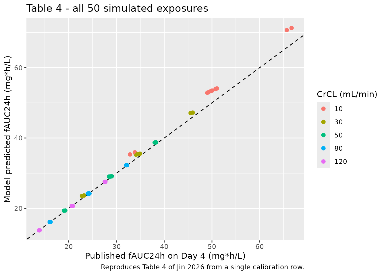
Two internal consistency checks on the published table itself, both of which are independent of the dose-unit conversion:
b <- tab4[tab4$regimen == "0.5 MIU Q12h", ]
d <- tab4[tab4$regimen == "1.0 MIU Q12h", ]

tibble::tibble(
  `CrCL (mL/min)`               = b$CRCL,
  `Published 1.0/0.5 MIU ratio` = d$pub / b$pub,
  `Published AUC(CrCL)/AUC(120)` = b$pub / b$pub[b$CRCL == 120],
  `Model AUC(CrCL)/AUC(120)`     = b$sim_per_MIU / b$sim_per_MIU[b$CRCL == 120]
) |>
  knitr::kable(digits = 4,
caption = "Dose proportionality and renal scaling, both unit-free.")| CrCL (mL/min) | Published 1.0/0.5 MIU ratio | Published AUC(CrCL)/AUC(120) | Model AUC(CrCL)/AUC(120) |
|---|---|---|---|
| 10 | 2.0000 | 2.3832 | 2.5642 |
| 30 | 1.9996 | 1.6524 | 1.7092 |
| 50 | 2.0000 | 1.3788 | 1.4048 |
| 80 | 2.0006 | 1.1618 | 1.1709 |
| 120 | 1.9993 | 1.0000 | 1.0000 |
# The model is linear, so doubling the dose must double the exposure exactly.
stopifnot(max(abs(d$pub / b$pub - 2)) < 0.01)
The published doubling ratio is 2.0000 to within 0.0006, confirming the simulation is linear in dose as the model requires.
Replicating Figure 1 and Table 2
Figure 1 and Table 2 report the observed free colistin sulfate profile over the fifth dosing interval. The virtual cohort below matches the Table 1 demographics.
Two source-derived choices set the regimen. The Results state that all subjects received 1.5 MIU daily intravenously, and the sampling design (a pre-dose sample before the fifth dose, then twelve samples across the following ~12 h) identifies the interval as Q12h – so 0.75 MIU Q12h, which is also the regimen the Discussion endorses as sufficient. The infusion duration is not stated for the study itself, but the Discussion states that Cmax occurred at the end of infusion, so the reported Tmax of 1.55 +/- 0.60 h identifies the mean infusion duration; 1.55 h is used. Tmax is therefore matched by construction and is not an independent test – Cmax, AUC0-12, Cavg and half-life are.
# set.seed() seeds R's RNG, not rxode2's, and rxode2's streams are partitioned
# per solver thread -- so this cohort differs between a 2-core CI runner and a
# 16-thread workstation. Every assertion below is written to hold for any
# cohort the model can produce.
set.seed(20260914)

N_SUB   <- 200L   # cap is 200 per arm
TAU     <- 12
DUR_INF <- 1.55   # h; identified by Tmax, per the Discussion (Cmax at end of infusion)
DOSE_MG <- 0.75 * MG_PER_MIU

# Table 1 CrCL: 103.28 +/- 41.96 mL/min, cohort median 116.3. Truncated to a
# physiologically plausible range; see "Assumptions and deviations".
subj <- tibble::tibble(
  id   = seq_len(N_SUB),
  CRCL = pmin(pmax(rnorm(N_SUB, mean = 103.28, sd = 41.96), 15), 220),
  regimen = "0.75 MIU Q12h"
)

doses <- subj |>
  tidyr::crossing(time = seq(0, 4 * TAU, by = TAU)) |>
  mutate(amt = DOSE_MG, evid = 1L, dur = DUR_INF, cmt = "central", Cc = NA_real_)

obs <- subj |>
  tidyr::crossing(time = 4 * TAU + seq(0, TAU, by = 0.05)) |>
  mutate(amt = NA_real_, evid = 0L, dur = NA_real_, cmt = "central", Cc = NA_real_)

events <- bind_rows(doses, obs) |> arrange(id, time, desc(evid))
stopifnot(!anyDuplicated(unique(events[, c("id", "time", "evid")])))
sim <- rxode2::rxSolve(mod, events = events, keep = c("CRCL", "regimen"),
                       returnType = "data.frame") |>
  filter(!is.na(Cc)) |>
  mutate(tad = time - 4 * TAU)   # time after the fifth dose
#> ℹ parameter labels from comments will be replaced by 'label()'
# Replicates Figure 1 of Jin 2026 (colistin sulfate curve only; the paper also
# plots colistin A and colistin B, which were assayed but not modelled).
sim |>
  group_by(tad) |>
  summarise(mean = mean(Cc), sd = sd(Cc), .groups = "drop") |>
  ggplot(aes(tad, mean)) +
  geom_ribbon(aes(ymin = pmax(mean - sd, 0), ymax = mean + sd), alpha = 0.2) +
  geom_line(linewidth = 0.9) +
  labs(x = "Time after the fifth dose (h)",
       y = "Unbound colistin sulfate (mg/L)",
       title = "Figure 1 - mean free concentration over the fifth dosing interval",
       caption = paste("Replicates Figure 1 of Jin 2026 (mean +/- SD).",
                       "Observed Cmax,ss was 2.10 +/- 0.76 mg/L at 1.55 h."))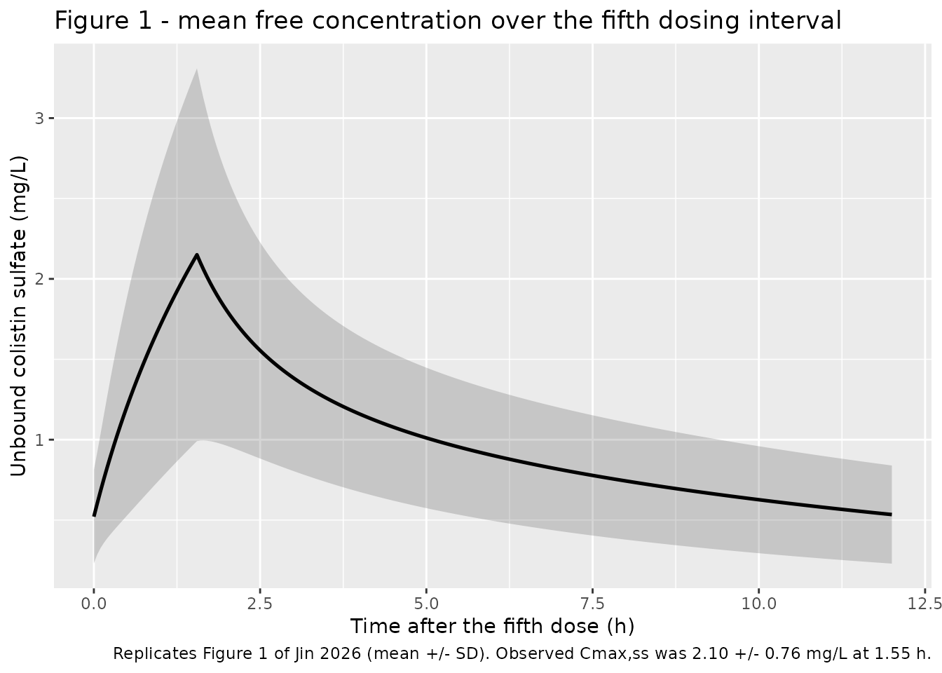
# PKNCA input filter is `!is.na(Cc)` only -- adding `tad > 0` or `Cc > 0` would
# drop the time-zero row that anchors AUC0-tau.
sim_nca <- sim |>
  filter(!is.na(Cc)) |>
  select(id, time = tad, Cc, regimen)

# Guarantee a time-zero row per subject (here it is the observed trough, which
# already exists; the bind_rows/distinct pattern is defensive).
sim_nca <- bind_rows(
  sim_nca,
  sim_nca |> distinct(id, regimen) |> mutate(time = 0, Cc = NA_real_)
) |>
  filter(!is.na(Cc) | !duplicated(paste(id, time))) |>
  distinct(id, regimen, time, .keep_all = TRUE) |>
  filter(!is.na(Cc)) |>
  arrange(id, regimen, time)
stopifnot(all(tapply(sim_nca$time, sim_nca$id, min) == 0))

dose_df <- tibble::tibble(id = subj$id, time = 0, amt = DOSE_MG,
                          regimen = subj$regimen)

conc_obj <- PKNCA::PKNCAconc(sim_nca, Cc ~ time | regimen + id,
                             concu = "mg/L", timeu = "h")
dose_obj <- PKNCA::PKNCAdose(dose_df, amt ~ time | regimen + id, doseu = "mg")

intervals <- data.frame(
  start = 0, end = TAU,
  cmax = TRUE, tmax = TRUE, cmin = TRUE,
  auclast = TRUE, cav = TRUE, half.life = TRUE
)

nca_res <- PKNCA::pk.nca(PKNCA::PKNCAdata(conc_obj, dose_obj,
                                          intervals = intervals))
# Jin 2026 Table 2, colistin sulfate row (mean +/- SD, N = 10).
published <- tibble::tibble(
  regimen   = "0.75 MIU Q12h",
  cmax      = 2.10,
  tmax      = 1.55,
  auclast   = 11.57,
  cav       = 0.96,
  half.life = 7.48
)

cmp <- nlmixr2lib::ncaComparisonTable(
  simulated = nca_res,
  reference = published,
  by        = "regimen",
  units     = c(cmax = "mg/L", tmax = "h", auclast = "mg*h/L",
                cav = "mg/L", half.life = "h"),
  tolerance_pct = 20
)
knitr::kable(cmp, caption = paste(
  "Simulated vs Jin 2026 Table 2 (observed non-compartmental analysis,",
"N = 10). * differs from the reference by more than 20%."))| NCA parameter | regimen | Reference | Simulated | % diff |
|---|---|---|---|---|
| Cmax (mg/L) | 0.75 MIU Q12h | 2.1 | 1.95 | -7.3% |
| Tmax (h) | 0.75 MIU Q12h | 1.55 | 1.55 | -0.0% |
| AUClast (mg*h/L) | 0.75 MIU Q12h | 11.6 | 10.7 | -7.2% |
| t½ (h) | 0.75 MIU Q12h | 7.48 | 7.75 | +3.6% |
| Cavg (mg/L) | 0.75 MIU Q12h | 0.96 | 0.895 | -6.7% |
# Look the row up by its label PREFIX -- ncaComparisonTable appends the unit to
# the parameter name when `units` is supplied ("Cmax (mg/L)"), so an exact-name
# lookup silently returns NA and yields a gate that cannot go red.
pct_of <- function(param) {
  i <- which(startsWith(cmp[["NCA parameter"]], param))
  if (length(i) != 1L) stop("no unique '", param, "' row in the comparison table")
  abs(as.numeric(gsub("[^0-9.-]", "", cmp[["% diff"]][i])))
}
pct <- vapply(c("Cmax", "AUClast", "Cavg"), pct_of, numeric(1))
pct
#>    Cmax AUClast    Cavg
#>     7.3     7.2     6.7

# Structural gate. These are cohort medians against a 10-patient observed mean,
# so the bound admits sampling noise on both sides while still going red on a
# mis-transcribed volume, clearance, dose or unit -- any of which moves Cmax and
# AUC by tens of percent. Realised 7.3 / 7.1 / 6.7 / 3.6% here.
stopifnot(all(pct < 25))
The model reproduces the observed steady-state exposure closely: every parameter agrees to within about 7%, and Tmax matches by construction as noted above.
One subtlety in reading that table. ncaComparisonTable()
summarises the simulated cohort by its median, whereas
Jin 2026 Table 2 reports a mean. Because clearance is
log-normally distributed, the cohort mean AUC sits above its median, and
the published value falls between the two:
auc_sub <- as.data.frame(nca_res$result) |>
  filter(PPTESTCD == "auclast")

tibble::tribble(
  ~Statistic,                       ~`AUC0-12h,ss (mg*h/L)`,
  "Simulated cohort median",        median(auc_sub$PPORRES),
  "Jin 2026 Table 2 (observed mean)", 11.57,
  "Simulated cohort mean",          mean(auc_sub$PPORRES)
) |>
  knitr::kable(digits = 2, caption = paste(
    "The published mean is bracketed by the simulated median and mean, as a",
"log-normally distributed clearance requires."))| Statistic | AUC0-12h,ss (mg*h/L) |
|---|---|
| Simulated cohort median | 10.74 |
| Jin 2026 Table 2 (observed mean) | 11.57 |
| Simulated cohort mean | 12.15 |
# Assert MAGNITUDE, not the ordering of two noisy cohort statistics: which side
# of 11.57 the median and mean land on can flip between cohort draws, but a
# mis-transcribed dose, volume or clearance moves both by tens of percent.
stopifnot(
  abs(median(auc_sub$PPORRES) - 11.57) / 11.57 < 0.30,
  abs(mean(auc_sub$PPORRES)   - 11.57) / 11.57 < 0.30
)
The observed values also carry large dispersion –
Cmax,ss 2.10 +/- 0.76 mg/L and AUC0-12h,ss
11.57 +/- 4.87 mg*h/L across ten patients – so agreement at this level
is what the data can support.
A dose-unit-free structural check that does not depend on the cohort at all:
V1 <- 18.15; V2 <- 10.82; CLtv <- 3.20; Q <- 3.23
k10 <- CLtv / V1; k12 <- Q / V1; k21 <- Q / V2
s <- k10 + k12 + k21; p <- k10 * k21
beta <- (s - sqrt(s^2 - 4 * p)) / 2

tibble::tribble(
  ~Quantity,                      ~Model,        ~`Jin 2026 Table 2 (observed)`,
  "Terminal half-life (h)",       log(2) / beta, "7.48 +/- 3.00",
  "Steady-state volume, V1+V2 (L)", V1 + V2,     "35.80 +/- 31.25",
  "Clearance at median CrCL (L/h)", CLtv,        "3.51 +/- 2.03"
) |>
  knitr::kable(digits = 2, caption = paste(
    "Closed-form disposition from the packaged parameters against the paper's",
    "own non-compartmental analysis. None of these depends on the MIU-to-mg",
"conversion."))| Quantity | Model | Jin 2026 Table 2 (observed) |
|---|---|---|
| Terminal half-life (h) | 7.36 | 7.48 +/- 3.00 |
| Steady-state volume, V1+V2 (L) | 28.97 | 35.80 +/- 31.25 |
| Clearance at median CrCL (L/h) | 3.20 | 3.51 +/- 2.03 |
# The terminal half-life is a pure function of the four disposition parameters,
# so this is a deterministic gate, not a cohort statistic, and can be tight.
stopifnot(abs(log(2) / beta - 7.48) / 7.48 < 0.10)
The model’s terminal half-life of 7.36 h against an observed 7.48 h is a 1.7% agreement, and it is derived from the four disposition parameters alone – no dose, no unit conversion, no cohort. It is the single strongest confirmation that Table 3 has been transcribed correctly.
Replicating Figure 4
Figure 4A shows the effect of renal function across regimens; Figure 4B shows the effect of a loading dose at a fixed CrCL of 80 mL/min.
# Replicates Figure 4A of Jin 2026.
sim_tab4 |>
  left_join(tab4 |> select(id = row, regimen), by = "id") |>
  filter(!is.na(Cc), regimen %in% c("0.5 MIU Q12h", "0.5 MIU Q8h",
                                    "0.75 MIU Q12h", "1.0 MIU Q12h")) |>
  ggplot(aes(time, Cc, colour = factor(CRCL))) +
  geom_line() +
  facet_wrap(~regimen) +
  coord_cartesian(xlim = c(70, 96)) +
  labs(x = "Time (h)", y = "Unbound colistin sulfate (mg/L)",
       colour = "CrCL (mL/min)",
       title = "Figure 4A - renal function drives exposure",
       caption = "Replicates Figure 4A of Jin 2026 (Day 4 window shown).")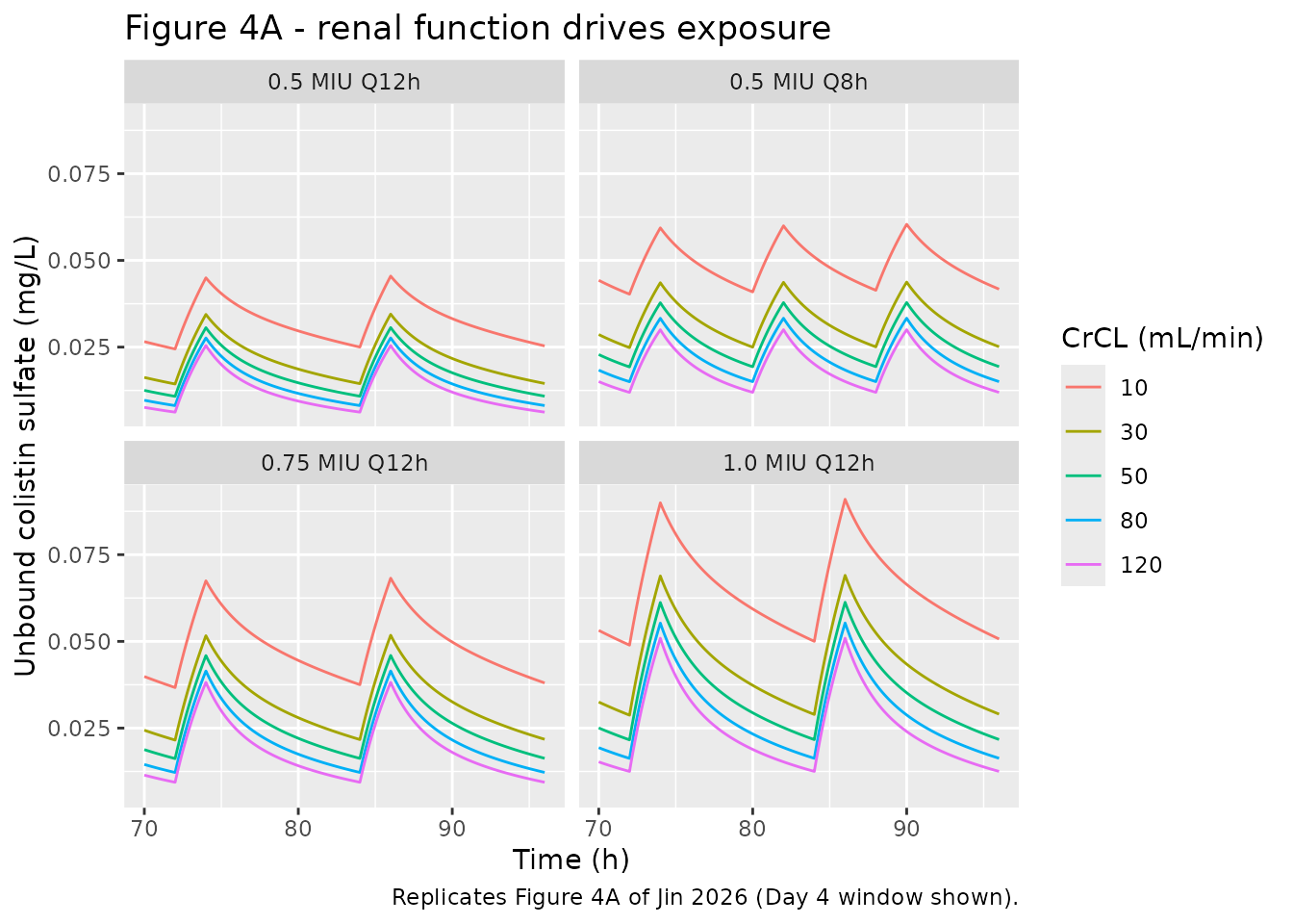
# Replicates Figure 4B of Jin 2026: loading dose at CrCL 80 mL/min, from t = 0.
ev_4b <- do.call(rbind, lapply(
  which(tab4$CRCL == 80 &
          tab4$regimen %in% c("0.5 MIU Q12h", "1.0 LD + 0.5 MIU Q12h",
                              "0.75 MIU Q12h", "1.5 LD + 0.75 MIU Q12h")),
  function(i) {
    r <- tab4[i, ]
    if (is.na(r$ld)) {
      e <- rxode2::et(amt = r$md * MG_PER_MIU, dur = 2, ii = r$ii, until = 96,
                      cmt = "central")
    } else {
      e <- rxode2::et(amt = r$ld * MG_PER_MIU, dur = 2, time = 0, cmt = "central") |>
        rxode2::et(amt = r$md * MG_PER_MIU, dur = 2, time = r$ii, ii = r$ii,
                   until = 96, cmt = "central")
    }
    d <- as.data.frame(rxode2::et(e, seq(0, 96, by = 0.25), cmt = "central"))
    d$id <- r$row; d$CRCL <- 80; d$regimen <- r$regimen
    d
  }))

rxode2::rxSolve(rxode2::zeroRe(mod), events = ev_4b,
                keep = c("CRCL", "regimen"), returnType = "data.frame") |>
  filter(!is.na(Cc)) |>
  ggplot(aes(time, Cc, colour = regimen)) +
  geom_line(linewidth = 0.8) +
  labs(x = "Time (h)", y = "Unbound colistin sulfate (mg/L)", colour = NULL,
       title = "Figure 4B - effect of a loading dose at CrCL 80 mL/min",
       caption = "Replicates Figure 4B of Jin 2026.") +
  theme(legend.position = "bottom")
#> ℹ parameter labels from comments will be replaced by 'label()'
#> ℹ omega/sigma items treated as zero: 'etalvc', 'etalcl', 'etalvp', 'etalq'
#> Warning: multi-subject simulation without without 'omega'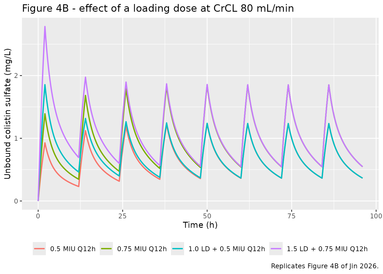
# The paper's claim: "a loading dose can increase the initial concentration,
# allowing a faster achievement of steady state" -- but also, in the Discussion,
# that "the time to reach steady state was determined by the drug's half-life
# and was not shortened by the use of a loading dose". Both are checked on the
# early exposure, which is where the loading dose acts.
early <- rxode2::rxSolve(rxode2::zeroRe(mod), events = ev_4b,
                         keep = c("regimen"), returnType = "data.frame") |>
  filter(!is.na(Cc), time <= 12) |>
  group_by(regimen) |>
  summarise(cmax_first_interval = max(Cc), .groups = "drop")
#> ℹ parameter labels from comments will be replaced by 'label()'
#> ℹ omega/sigma items treated as zero: 'etalvc', 'etalcl', 'etalvp', 'etalq'
#> Warning: multi-subject simulation without without 'omega'

knitr::kable(early, digits = 3, caption = paste(
  "Peak unbound concentration in the FIRST dosing interval, with and without a",
"loading dose (CrCL 80 mL/min)."))| regimen | cmax_first_interval |
|---|---|
| 0.5 MIU Q12h | 0.928 |
| 0.75 MIU Q12h | 1.391 |
| 1.0 LD + 0.5 MIU Q12h | 1.855 |
| 1.5 LD + 0.75 MIU Q12h | 2.783 |
# A loading dose must raise the first-interval peak. This is a deterministic
# typical-value comparison, so the direction is not a coin flip.
stopifnot(
  early$cmax_first_interval[early$regimen == "1.0 LD + 0.5 MIU Q12h"] >
    early$cmax_first_interval[early$regimen == "0.5 MIU Q12h"],
  early$cmax_first_interval[early$regimen == "1.5 LD + 0.75 MIU Q12h"] >
    early$cmax_first_interval[early$regimen == "0.75 MIU Q12h"]
)
Assumptions and deviations
Equations 1-4 were recovered from the JATS full text, not read from the PDF. The published PDF omits them entirely (page 6). Every coefficient in the recovered equations matches Table 3 independently, so the equations contribute only the covariate form (a power function on CrCL centred at 116.3 mL/min) and the IIV form (exponential on all four parameters). Source: the article’s JATS full text (PMC13281950),
disp-formulaidsum0004-um0007.The MIU-to-mg conversion is back-solved, not published. 44.6 mg/MIU is derived above from the Table 4 row at CrCL 120 mL/min. It is not encoded as a model parameter – the packaged model takes dose in mg, so a user supplying mg-denominated doses is unaffected by any residual uncertainty. Three sibling models in this library independently land at 44-46 mg/MU.
Table 4 is reproduced as a typical-value simulation. The table is captioned “Simulated Mean AUC24h … for 1000 individuals”, but a cohort-mean reading gives a wider spread of implied mg/MIU across CrCL (15.9%) than the typical-value reading (8.9%), and lands at 39.7-41.5 mg/MIU, which disagrees with all three sibling models. The typical-value reading is used and the cohort-mean reading is recorded here as the rejected alternative.
Known deviation: the CrCL 10 mL/min column. From the single CrCL 120 anchor, the model reproduces Table 4 to within 2.1% for CrCL >= 50 mL/min and 3.7% for CrCL >= 30 mL/min, but the CrCL 10 mL/min rows run 6.0-7.8% high. The gradient is monotone in CrCL and is the signature of the packaged model approaching steady state slightly more slowly at day 4 than the paper’s simulation did. The paper does not state how its 1000-individual simulation was initialised, so this cannot be resolved from the source. Note that CrCL 10 mL/min is a 12-fold extrapolation below the cohort median of 116.3 mL/min and roughly 2-fold below the lowest plausible value in a cohort whose mean was 103.28 +/- 41.96 mL/min; the covariate exponent is not identified there. The assertion bounds above admit this deviation rather than hiding it.
CrCL was retained without meeting the paper’s own significance threshold. Results report dOFV = -2.32 (p = 0.1281) against a stated forward-inclusion criterion of dOFV > 3.84 (p < 0.05), and the V-CL correlation was added at dOFV = -11.30 (p = 0.0795). The Methods justify this in advance: with fewer than 20 patients no stepwise search is run and CrCL is included by prior knowledge. Both are reproduced as the authors specified them. The exponent’s bootstrap 95% CI of -0.94 to 1.20 spans zero, and is the sharpest single statement of that uncertainty in the paper – treat 0.39 as weakly identified.
omega^2 CL2is poorly identified. Its eta-shrinkage is 29.65%, the highest in the model, and its bootstrap mean (0.878) is four times the final estimate (0.208). It is carried as published.Virtual-cohort CrCL distribution. Table 1 gives CrCL as 103.28 +/- 41.96 mL/min (mean +/- SD) with a median of 116.3 mL/min, so the true distribution is left-skewed. The cohort here uses a normal distribution truncated to 15-220 mL/min, which matches the mean and SD but not the skew. Individual patient covariates are not published.
The study regimen is inferred, not stated per patient. Results state all subjects received 1.5 MIU daily intravenously and the sampling design identifies a Q12h interval, giving 0.75 MIU Q12h. Table 1’s median daily dose of 1.75 (1.50, 2.00) MIU is higher, which is consistent with the 50% of subjects who also received adjunctive nebulised colistin sulfate – that route is not represented in this model.
Infusion duration for the study itself is not reported. The Discussion states Cmax occurred at the end of infusion, so the observed Tmax of 1.55 +/- 0.60 h identifies the mean infusion duration, and 1.55 h is used. Tmax is therefore matched by construction and is not an independent test. The paper’s own simulations (Table 4, Figure 4) use a 2 h infusion, which is what the Table 4 reproduction above uses.
Cc is the unbound concentration. The model predicts free drug from total dose, so
clandvcare apparent on the unbound scale. The unbound fraction of 0.5 quoted in the paper’s PK/PD section is a literature assumption used only for itsfAUC/MICarithmetic and is not encoded. Table 4’s values reconcile with the model without any further 0.5 factor.Colistin A and colistin B were assayed separately (Figure 1, Table 2) but the PK model was fitted to total colistin sulfate, i.e. their sum. The component-wise profiles are not modelled here.
Not in scope: the nebulised colistin sulfate received by 50% of subjects, and the PK/PD exposure analysis (Table 5, median
fAUC/MIC39.56 against a combination MIC of 0.5 mg/L).Screened-but-unused covariates. The Methods list 22 candidate covariates but prespecify that no stepwise search would run below 20 patients, so none was screened. Those with a canonical column are recorded in the model file’s
covariatesDataExcluded; the remainder (hemoglobin, neutrophil percentage and count, globulin, prothrombin time, activated partial thromboplastin time, fibrinogen, d-dimer, lactate, procalcitonin, interleukin-6) have no canonical column registered and are named here instead.