Abemaciclib CDK4/6 occupancy and pRB / TOPO-IIa biomarker QSP (Zhang 2025)

Model and source

• Citation: Zhang C, Li S, Ren J, Lang R. (2025). Physiologically Based Pharmacokinetic Model of Plasma and Intracranial Pharmacokinetics and CDK4/6 Occupancy of Abemaciclib to Optimizing Dosing Regimen for Brain Metastatic Patients. ACS Omega 10(9):9245-9256. doi:10.1021/acsomega.4c09472. PMCID PMC11904693. Target-engagement equation from Methods 2.1 (Eq 1, after Wong 2019); fraction-unbound albumin scaling from Methods 2.1 (Eq 2, after Alsmadi 2021); biomarker chain from Methods 2.2 (Eqs 4-7, framework from Tate 2014). All parameter values are from main-text Table 1. Note that the trimmed markdown companion of this paper retains Table 1 and Section 3.6 but drops every display equation (eight ‘formula-not-decoded’ markers), so Eqs 1-7 were recovered from the PDF.
• Article (open access, CC BY-NC-ND 4.0): https://doi.org/10.1021/acsomega.4c09472
• PMC record: https://www.ncbi.nlm.nih.gov/pmc/articles/PMC11904693/

mod <- readModelDb("Zhang_2025_abemaciclib_qsp")
ui  <- rxode2::rxode2(mod)
mod
#> function() {
#>   description <- paste(
#>     "QSP. CDK4/6 target-engagement and pRB / TOPO-IIa cell-cycle biomarker model",
#>     "for abemaciclib (ABE) and its three active metabolites M2, M18 and M20 in",
#>     "patients with metastatic breast cancer, including brain metastases. Four",
#>     "analytes compete reversibly for a shared CDK4 pool and a shared CDK6 pool",
#>     "(0.1 uM each) in plasma and in cerebrospinal fluid, and the resulting CDK",
#>     "occupancy fraction drives a four-compartment cell-cycle transit chain",
#>     "(early G1 precursor, late G1 pRB, S-phase TOPO-IIa, G2M) whose framework",
#>     "comes from Tate 2014. The abemaciclib and metabolite concentrations are NOT",
#>     "fitted here: Zhang 2025 generated them with a whole-body PK-Sim 9.1 PBPK",
#>     "model that is a platform port (system-specific parameters were taken from",
#>     "the built-in PK-Sim database, distribution used the built-in Rodgers and",
#>     "Rowland method, no organ ODEs / volumes / blood flows are published and no",
#>     ".pksim5 project was deposited), so that layer is not reproducible from the",
#>     "on-disk sources and is deliberately NOT extracted. Total plasma",
#>     "concentrations are instead supplied per record as the canonical",
#>     "time-varying covariates CP_ABE_NGML, CP_M2_NGML, CP_M18_NGML and",
#>     "CP_M20_NGML, and the albumin-scaled fraction unbound is applied inside",
#>     "model(), following the Liang_2024_osimertinib_qsp precedent. Deterministic",
#>     "mechanism model: Zhang 2025 propagated variability through PK-Sim virtual",
#>     "population physiology rather than fitting IIV or residual error, so no etas",
#>     "and no error model are encoded. The CSF limb applies the fixed Table 1",
#>     "CSF-to-plasma ratio K_CSF,p to the free plasma concentration, exactly as",
#>     "Methods 2.1 describes. Validated against the paper's own prose claims, the",
#>     "model reproduces five of the six numeric statements in Section 3.6,",
#>     "including both 150 mg BID claims (CSF CDK4 above 90%, CSF CDK6 above 80%);",
#>     "the one it misses is CSF CDK6 above 90% at 200 mg BID, where it returns",
#>     "about 86%. That shortfall is small and is not necessarily structural: the",
#>     "analyte concentrations used to score it are reconstructed from Table 2 plus",
#>     "the published metabolite mass split rather than taken from the",
#>     "un-extracted PBPK layer, and that reconstruction is itself about 17% low",
#>     "against the paper's own quoted total-analyte trough. See the vignette",
#>     "'Assumptions and deviations' section, which quantifies both candidate",
#>     "causes.",
#>     sep = " "
#>   )
#>   reference <- paste(
#>     "Zhang C, Li S, Ren J, Lang R. (2025). Physiologically Based Pharmacokinetic",
#>     "Model of Plasma and Intracranial Pharmacokinetics and CDK4/6 Occupancy of",
#>     "Abemaciclib to Optimizing Dosing Regimen for Brain Metastatic Patients.",
#>     "ACS Omega 10(9):9245-9256. doi:10.1021/acsomega.4c09472. PMCID PMC11904693.",
#>     "Target-engagement equation from Methods 2.1 (Eq 1, after Wong 2019);",
#>     "fraction-unbound albumin scaling from Methods 2.1 (Eq 2, after Alsmadi",
#>     "2021); biomarker chain from Methods 2.2 (Eqs 4-7, framework from Tate",
#>     "2014). All parameter values are from main-text Table 1. Note that the",
#>     "trimmed markdown companion of this paper retains Table 1 and Section 3.6",
#>     "but drops every display equation (eight 'formula-not-decoded' markers), so",
#>     "Eqs 1-7 were recovered from the PDF.",
#>     sep = " "
#>   )
#>   vignette <- "Zhang_2025_abemaciclib"
#> 
#>   units <- list(
#>     time          = "h",
#>     dosing        = "(not applicable; the analyte concentrations are supplied as the time-varying covariates CP_ABE_NGML, CP_M2_NGML, CP_M18_NGML and CP_M20_NGML)",
#>     concentration = "nmol/L"
#>   )
#> 
#>   # The bound drug-CDK complexes are indexed by kinase isoform (CDK4 / CDK6),
#>   # by analyte (parent + three metabolites) and by matrix (plasma / CSF), which
#>   # the canonical bare `complex` name cannot express. Declared here rather than
#>   # silently warned on, following the Liang_2024_osimertinib_qsp precedent.
#>   # `precursor`, `prb` and `topo2a` are the cell-cycle transit states of Eqs 4-6.
#>   paper_specific_compartments <- c(
#>     "complex_cdk4_abe",     "complex_cdk4_m2",     "complex_cdk4_m18",     "complex_cdk4_m20",
#>     "complex_cdk6_abe",     "complex_cdk6_m2",     "complex_cdk6_m18",     "complex_cdk6_m20",
#>     "complex_cdk4_abe_csf", "complex_cdk4_m2_csf", "complex_cdk4_m18_csf", "complex_cdk4_m20_csf",
#>     "complex_cdk6_abe_csf", "complex_cdk6_m2_csf", "complex_cdk6_m18_csf", "complex_cdk6_m20_csf",
#>     "precursor", "prb", "topo2a"
#>   )
#> 
#>   # Issue #482: what each ODE state holds, in what amount units, in what
#>   # biological matrix. The occupancy states are molar concentrations of the
#>   # drug-CDK complex (the CDK pools are declared as 0.1 uM concentrations, not
#>   # amounts). The three biomarker states are dimensionless expression levels
#>   # relative to the untreated baseline (see the `prb0` note in ini()).
#>   compartmentData <- list(
#>     complex_cdk4_abe     = list(analyte = "abemaciclib-CDK4 complex",  units = "nmol/L", specimen = "plasma", verified = TRUE),
#>     complex_cdk4_m2      = list(analyte = "M2-CDK4 complex",           units = "nmol/L", specimen = "plasma", verified = TRUE),
#>     complex_cdk4_m18     = list(analyte = "M18-CDK4 complex",          units = "nmol/L", specimen = "plasma", verified = TRUE),
#>     complex_cdk4_m20     = list(analyte = "M20-CDK4 complex",          units = "nmol/L", specimen = "plasma", verified = TRUE),
#>     complex_cdk6_abe     = list(analyte = "abemaciclib-CDK6 complex",  units = "nmol/L", specimen = "plasma", verified = TRUE),
#>     complex_cdk6_m2      = list(analyte = "M2-CDK6 complex",           units = "nmol/L", specimen = "plasma", verified = TRUE),
#>     complex_cdk6_m18     = list(analyte = "M18-CDK6 complex",          units = "nmol/L", specimen = "plasma", verified = TRUE),
#>     complex_cdk6_m20     = list(analyte = "M20-CDK6 complex",          units = "nmol/L", specimen = "plasma", verified = TRUE),
#>     complex_cdk4_abe_csf = list(analyte = "abemaciclib-CDK4 complex",  units = "nmol/L", specimen = "CSF", verified = TRUE),
#>     complex_cdk4_m2_csf  = list(analyte = "M2-CDK4 complex",           units = "nmol/L", specimen = "CSF", verified = TRUE),
#>     complex_cdk4_m18_csf = list(analyte = "M18-CDK4 complex",          units = "nmol/L", specimen = "CSF", verified = TRUE),
#>     complex_cdk4_m20_csf = list(analyte = "M20-CDK4 complex",          units = "nmol/L", specimen = "CSF", verified = TRUE),
#>     complex_cdk6_abe_csf = list(analyte = "abemaciclib-CDK6 complex",  units = "nmol/L", specimen = "CSF", verified = TRUE),
#>     complex_cdk6_m2_csf  = list(analyte = "M2-CDK6 complex",           units = "nmol/L", specimen = "CSF", verified = TRUE),
#>     complex_cdk6_m18_csf = list(analyte = "M18-CDK6 complex",          units = "nmol/L", specimen = "CSF", verified = TRUE),
#>     complex_cdk6_m20_csf = list(analyte = "M20-CDK6 complex",          units = "nmol/L", specimen = "CSF", verified = TRUE),
#>     # The biomarker matrix is SKIN, not tumor -- Zhang 2025 says so explicitly in
#>     # the Discussion: "it is noteworthy that the biomarker model predicts changes
#>     # in pRB and TOPO-IIa occurring in skin tissue, rather than in tumor tissue.
#>     # Because the only alterations in pRB and TOPO-IIa within skin tissue in
#>     # humans has been experimentally determined, it is assumed that the
#>     # differences between the pRB and TOPO-IIa biomarker expression in tumors and
#>     # skin tissue are negligible." The controlled specimen vocabulary
#>     # (R/conventions.R) has no `skin` term, so these carry the generic `tissue`
#>     # and name skin in `analyte`; recording `tumor` here would contradict the
#>     # source.
#>     precursor            = list(analyte = "cells accumulated in early G1 (precursor compartment PC), skin", units = "fraction of untreated baseline", specimen = "tissue", verified = TRUE),
#>     prb                  = list(analyte = "phosphorylated retinoblastoma protein (pRB) expression, skin",   units = "fraction of untreated baseline", specimen = "tissue", verified = TRUE),
#>     topo2a               = list(analyte = "topoisomerase-II alpha (TOPO-IIa) expression, skin",             units = "fraction of untreated baseline", specimen = "tissue", verified = TRUE)
#>   )
#> 
#>   covariateData <- list(
#>     CP_ABE_NGML = list(
#>       description        = "Time-varying TOTAL abemaciclib plasma concentration driving CDK4/6 engagement",
#>       units              = "ng/mL",
#>       type               = "continuous",
#>       reference_category = NULL,
#>       notes              = paste(
#>         "TOTAL (not free) plasma concentration. The free concentration that",
#>         "actually drives binding is computed inside model() as",
#>         "CP_ABE_NGML * fup_abe, with fup_abe scaled to the subject's albumin by",
#>         "the paper's Eq 2. Zhang 2025 Eq 1 defines its driver as 'the free drug",
#>         "concentration in plasma or the CSF'. Supplying a total concentration is",
#>         "the more useful convention because that is what a PK model returns.",
#>         "In the source study this concentration is produced by a whole-body",
#>         "PK-Sim 9.1 PBPK model that is not reproducible from the published",
#>         "sources and is not extracted (see description).",
#>         "Published steady-state anchors in patients (Zhang 2025 Table 2,",
#>         "predicted column, Patnaik 2016 regimens): Cmin 144 ng/mL and Cmax",
#>         "198 ng/mL at 100 mg BID; Cmin 174 and Cmax 250 at 150 mg BID; Cmin 231",
#>         "and Cmax 333 at 200 mg BID. Total active analytes (ABE + M2 + M20)",
#>         "reach a mean plasma Cmin of 498 ng/mL at the standard 200 mg BID",
#>         "regimen, against a stated safety ceiling of 693 ng/mL (Zhang 2025",
#>         "Sections 2.6 and 3.6)."
#>       ),
#>       source_name        = "(none; computed by the PK-Sim PBPK model, not a named NONMEM data column)"
#>     ),
#>     CP_M2_NGML = list(
#>       description        = "Time-varying TOTAL M2 (active abemaciclib metabolite) plasma concentration driving CDK4/6 engagement",
#>       units              = "ng/mL",
#>       type               = "continuous",
#>       reference_category = NULL,
#>       notes              = paste(
#>         "TOTAL plasma concentration of the active metabolite M2; the free",
#>         "concentration is CP_M2_NGML * fup_m2 inside model(). Zhang 2025",
#>         "Introduction (citing the FDA multidiscipline review, ref 14) reports",
#>         "that M2 contributes 13% of total plasma mass in vivo. Set to 0 to",
#>         "study the parent alone."
#>       ),
#>       source_name        = "(none; computed by the PK-Sim PBPK model, not a named NONMEM data column)"
#>     ),
#>     CP_M18_NGML = list(
#>       description        = "Time-varying TOTAL M18 (active abemaciclib metabolite) plasma concentration driving CDK4/6 engagement",
#>       units              = "ng/mL",
#>       type               = "continuous",
#>       reference_category = NULL,
#>       notes              = paste(
#>         "TOTAL plasma concentration of the active metabolite M18; the free",
#>         "concentration is CP_M18_NGML * fup_m18 inside model(). Zhang 2025",
#>         "Introduction (ref 14) reports that M18 contributes 5% of total plasma",
#>         "mass in vivo. M18 is the metabolite for which no CSF data existed, so",
#>         "its K_CSF,p was assumed to be 1.0 (Zhang 2025 Methods 2.1). Set to 0",
#>         "to study the parent alone."
#>       ),
#>       source_name        = "(none; computed by the PK-Sim PBPK model, not a named NONMEM data column)"
#>     ),
#>     CP_M20_NGML = list(
#>       description        = "Time-varying TOTAL M20 (active abemaciclib metabolite) plasma concentration driving CDK4/6 engagement",
#>       units              = "ng/mL",
#>       type               = "continuous",
#>       reference_category = NULL,
#>       notes              = paste(
#>         "TOTAL plasma concentration of the active metabolite M20; the free",
#>         "concentration is CP_M20_NGML * fup_m20 inside model(). Zhang 2025",
#>         "Introduction (ref 14) reports that M20 contributes 26% of total plasma",
#>         "mass in vivo, making it the largest metabolite contributor. Set to 0",
#>         "to study the parent alone."
#>       ),
#>       source_name        = "(none; computed by the PK-Sim PBPK model, not a named NONMEM data column)"
#>     ),
#>     ALB = list(
#>       description        = "Plasma albumin concentration; scales the fraction unbound of all four analytes through the paper's Eq 2",
#>       units              = "g/L",
#>       type               = "continuous",
#>       reference_category = NULL,
#>       notes              = paste(
#>         "Canonical SI units g/L. Zhang 2025 reports albumin in g/dL throughout",
#>         "(divide by 10): 3.1 g/dL = 31 g/L in breast-cancer patients versus",
#>         "4.5 g/dL = 45 g/L in healthy subjects (Table 1 and Methods 2.1, after",
#>         "Alsmadi 2021). The Table 1 fup values are the PATIENT values, i.e.",
#>         "they already correspond to ALB = 31 g/L, so setting ALB = 31 recovers",
#>         "them exactly. Zhang 2025 Methods 2.5 swept albumin over 1.0-6.0 g/dL",
#>         "(10-60 g/L) to reflect the physiological range in cancer patients;",
#>         "note that in the source paper that sweep changes exposure through the",
#>         "PBPK layer as well as through binding, whereas here only the binding",
#>         "limb is reproduced."
#>       ),
#>       source_name        = "albumin (g/dl) (Zhang 2025 Table 1, physiological block)"
#>     )
#>   )
#> 
#>   population <- list(
#>     species        = "human (in silico; PK-Sim virtual populations matched to published clinical cohorts)",
#>     n_subjects     = NA_integer_,
#>     n_studies      = 4L,
#>     age_range      = "51-63 years (means of the contributing cohorts; Patnaik 2016 median 60, range 44-73)",
#>     sex_female_pct = NA_real_,
#>     disease_state  = "metastatic breast cancer, including hormone-receptor-positive / HER2-negative brain metastases; validation cohorts also included non-small cell lung cancer and other solid tumors",
#>     dose_range     = "abemaciclib 100-400 mg once daily or twice daily; validation at 100 and 150 mg OD and 100, 150 and 200 mg BID; 200 mg BID is the standard regimen",
#>     regions        = "United States, Europe and Japan (the contributing clinical studies)",
#>     notes          = paste(
#>       "Virtual-population demographics were taken per scenario from the four",
#>       "clinical plasma-PK studies and two CSF-PK studies tabulated in Zhang",
#>       "2025 Table 2 (Patnaik 2016, Tolaney 2020, Fujiwara 2016, Kim 2018),",
#>       "with PK-Sim mean values substituted where a study did not report a",
#>       "characteristic. Cohort sizes per arm ranged from 3 to 72 subjects;",
#>       "female proportion ranged from 33% to 100% across arms, so no single",
#>       "value is recorded here.",
#>       "Disease physiology differs from healthy subjects in three respects that",
#>       "Zhang 2025 states explicitly (Methods 2.1, after Alsmadi 2021): CYP3A4",
#>       "expression 3.02 versus 4.32 uM, albumin 3.1 versus 4.5 g/dL, and",
#>       "hematocrit 0.33 versus 0.43. Only the albumin difference enters the",
#>       "layer extracted here, through Eq 2; the other two act on the",
#>       "un-extracted PBPK layer.",
#>       "The pRB and TOPO-IIa observations the biomarker model was verified",
#>       "against are SKIN-biopsy measurements from Patnaik 2016, not tumor",
#>       "biopsies: Zhang 2025 states in the Discussion that the biomarker model",
#>       "'predicts changes in pRB and TOPO-IIa occurring in skin tissue, rather",
#>       "than in tumor tissue', because only the skin-tissue alterations have",
#>       "been experimentally determined in humans, and that the tumor-versus-skin",
#>       "difference is assumed negligible. The same Discussion paragraph notes",
#>       "that the paper does NOT ultimately treat these two biomarkers as",
#>       "predictive of clinical response (inhibition was of similar magnitude at",
#>       "150 and 200 mg BID), and uses a CDK4/6 occupancy above 90% as the",
#>       "efficacy predictor instead."
#>     )
#>   )
#> 
#>   ini({
#>     # ======================================================================
#>     # Molecular weights -- used only to convert the ng/mL covariates to the
#>     # nmol/L scale on which Kd and the CDK pools are reported.
#>     # Zhang 2025 Table 1, physicochemical block (source: ref 31, Posada 2020).
#>     # ======================================================================
#>     mw_abe <- fixed(506.6)
#>     label("Molecular weight of abemaciclib (g/mol)")
#>     # Zhang 2025 Table 1, MW row, ABE column.
#> 
#>     mw_m2 <- fixed(478.5)
#>     label("Molecular weight of metabolite M2 (g/mol)")
#>     # Zhang 2025 Table 1, MW row, M2 column.
#> 
#>     mw_m18 <- fixed(494.5)
#>     label("Molecular weight of metabolite M18 (g/mol)")
#>     # Zhang 2025 Table 1, MW row, M18 column.
#> 
#>     mw_m20 <- fixed(522.6)
#>     label("Molecular weight of metabolite M20 (g/mol)")
#>     # Zhang 2025 Table 1, MW row, M20 column.
#> 
#>     # ======================================================================
#>     # Fraction unbound in plasma, at the reference (patient) albumin level.
#>     # Zhang 2025 Table 1 fup row: "calculated using eq 2, original data was
#>     # from ref14". These are therefore the PATIENT values, i.e. the values at
#>     # albumin 3.1 g/dL, and model() re-scales them to any other albumin with
#>     # the same Eq 2 (see the algebra in the model() comment).
#>     # ======================================================================
#>     fup_abe <- fixed(0.039)
#>     label("Fraction of abemaciclib unbound in plasma at the reference albumin of 3.1 g/dL (unitless)")
#>     # Zhang 2025 Table 1, f_up row, ABE column.
#> 
#>     fup_m2 <- fixed(0.093)
#>     label("Fraction of M2 unbound in plasma at the reference albumin of 3.1 g/dL (unitless)")
#>     # Zhang 2025 Table 1, f_up row, M2 column.
#> 
#>     fup_m18 <- fixed(0.046)
#>     label("Fraction of M18 unbound in plasma at the reference albumin of 3.1 g/dL (unitless)")
#>     # Zhang 2025 Table 1, f_up row, M18 column.
#> 
#>     fup_m20 <- fixed(0.030)
#>     label("Fraction of M20 unbound in plasma at the reference albumin of 3.1 g/dL (unitless)")
#>     # Zhang 2025 Table 1, f_up row, M20 column.
#> 
#>     alb_ref <- fixed(31)
#>     label("Reference plasma albumin at which the fup values above apply (g/L; 3.1 g/dL in the source)")
#>     # Zhang 2025 Table 1, physiological block: "albumin (g/dl) 3.1", described
#>     # in Methods 2.1 as the mean value in patients (ref 30, Alsmadi 2021).
#> 
#>     # ======================================================================
#>     # CSF-to-plasma ratio of the FREE concentration. Zhang 2025 Methods 2.1:
#>     # 0.68 for ABE ("the mean ratio of ABE free concentration between the CSF
#>     # and plasma", ref 16), 0.14 for M2 and 0.91 for M20 (ref 33), and 1.0
#>     # assumed for M18 because no data were available.
#>     # ======================================================================
#>     kcsf_abe <- fixed(0.68)
#>     label("CSF-to-plasma free-concentration ratio for abemaciclib (unitless)")
#>     # Zhang 2025 Table 1, K_CSF,P row, ABE column; Methods 2.1.
#> 
#>     kcsf_m2 <- fixed(0.14)
#>     label("CSF-to-plasma free-concentration ratio for M2 (unitless)")
#>     # Zhang 2025 Table 1, K_CSF,P row, M2 column; Methods 2.1.
#> 
#>     kcsf_m18 <- fixed(1.0)
#>     label("CSF-to-plasma free-concentration ratio for M18 (unitless; assumed, no data available)")
#>     # Zhang 2025 Methods 2.1: "as no data were available for M18, KCSF,p was
#>     # assumed to be 1.0 for this metabolite." Table 1, K_CSF,P row, M18 column.
#> 
#>     kcsf_m20 <- fixed(0.91)
#>     label("CSF-to-plasma free-concentration ratio for M20 (unitless)")
#>     # Zhang 2025 Table 1, K_CSF,P row, M20 column; Methods 2.1.
#> 
#>     # ======================================================================
#>     # Equilibrium dissociation constants, one per analyte per kinase isoform.
#>     # Zhang 2025 Table 1 reports them as paired "CDK4/CDK6" entries; source
#>     # column: "ref15 for three metabolites and ref35 for ABE".
#>     # ======================================================================
#>     kd4_abe <- fixed(0.6)
#>     label("Equilibrium dissociation constant of abemaciclib for CDK4 (nmol/L)")
#>     # Zhang 2025 Table 1, Kd for CDK4/6 row, ABE column, first of the pair 0.6/8.2.
#> 
#>     kd6_abe <- fixed(8.2)
#>     label("Equilibrium dissociation constant of abemaciclib for CDK6 (nmol/L)")
#>     # Zhang 2025 Table 1, Kd for CDK4/6 row, ABE column, second of the pair 0.6/8.2.
#> 
#>     kd4_m2 <- fixed(1.2)
#>     label("Equilibrium dissociation constant of M2 for CDK4 (nmol/L)")
#>     # Zhang 2025 Table 1, Kd for CDK4/6 row, M2 column, pair 1.2/1.3.
#> 
#>     kd6_m2 <- fixed(1.3)
#>     label("Equilibrium dissociation constant of M2 for CDK6 (nmol/L)")
#>     # Zhang 2025 Table 1, Kd for CDK4/6 row, M2 column, pair 1.2/1.3.
#> 
#>     kd4_m18 <- fixed(1.2)
#>     label("Equilibrium dissociation constant of M18 for CDK4 (nmol/L)")
#>     # Zhang 2025 Table 1, Kd for CDK4/6 row, M18 column, pair 1.2/2.7.
#> 
#>     kd6_m18 <- fixed(2.7)
#>     label("Equilibrium dissociation constant of M18 for CDK6 (nmol/L)")
#>     # Zhang 2025 Table 1, Kd for CDK4/6 row, M18 column, pair 1.2/2.7.
#> 
#>     kd4_m20 <- fixed(1.5)
#>     label("Equilibrium dissociation constant of M20 for CDK4 (nmol/L)")
#>     # Zhang 2025 Table 1, Kd for CDK4/6 row, M20 column, pair 1.5/1.9.
#> 
#>     kd6_m20 <- fixed(1.9)
#>     label("Equilibrium dissociation constant of M20 for CDK6 (nmol/L)")
#>     # Zhang 2025 Table 1, Kd for CDK4/6 row, M20 column, pair 1.5/1.9.
#> 
#>     # ======================================================================
#>     # Dissociation rate constant and starting CDK expression.
#>     # ======================================================================
#>     koff <- fixed(6.0)
#>     label("First-order dissociation rate constant of the drug-CDK complex (1/h)")
#>     # Zhang 2025 Table 1, koff row: 0.10 /min, "fitted through nonlinear
#>     # analysis using the data from ref 36 for ABE, three metabolites were
#>     # assumed to be identical". Converted to the model time base of hours:
#>     # 0.10 /min * 60 min/h = 6.0 /h. A single koff applies to all four
#>     # analytes and to both isoforms.
#> 
#>     cdk0 <- fixed(100)
#>     label("Starting expression of each CDK isoform, CDK4/6_0 (nmol/L)")
#>     # Zhang 2025 Methods 2.1: "The starting expression of CDK4/6 (CDK4/60) was
#>     # set at default 0.1 uM due to not reported data in human." 0.1 uM = 100
#>     # nmol/L. Applied to the CDK4 pool and to the CDK6 pool separately, in
#>     # plasma and in CSF, because the paper reports the four occupancies
#>     # separately throughout (Figure 4 legend; every panel of Figure 5).
#> 
#>     # ======================================================================
#>     # Biomarker (cell-cycle transit) rate constants. Zhang 2025 Table 1,
#>     # biomarker block, source column: "kTo and kTo were optimized based on the
#>     # clinical study data, ref16; The remaining rate constants were taken from
#>     # the ref37" (Tate 2014).
#>     # ======================================================================
#>     krb <- fixed(0.16)
#>     label("Rate constant from early G1 to late G1, k_pRB (1/h)")
#>     # Zhang 2025 Table 1, kRB row.
#> 
#>     kto <- fixed(0.14)
#>     label("Rate constant from late G1 to S phase, k_TOPO-IIa (1/h)")
#>     # Zhang 2025 Table 1, kTO row.
#> 
#>     khh <- fixed(0.21)
#>     label("Rate constant from S phase to G2M phase, k_HH (1/h)")
#>     # Zhang 2025 Table 1, kHH row.
#> 
#>     kel_pc <- fixed(0.05)
#>     label("Elimination rate constant from the early-G1 precursor compartment (1/h)")
#>     # Zhang 2025 Table 1, kel row (units not printed in Table 1; 1/h by
#>     # consistency with the other three rate constants in the same block and
#>     # with Eq 7, in which kel is summed with k_pRB).
#> 
#>     prb0 <- fixed(1)
#>     label("Baseline pRB expression scale factor (fraction of untreated baseline)")
#>     # Zhang 2025 Eq 7 defines k_in = pRB0 * (k_pRB + k_el) and says only that
#>     # "pRB0 is the baseline expression in patients" (ref 16); no numeric value
#>     # is printed anywhere in the paper or Table 1. Setting it to 1 is EXACT
#>     # rather than an assumption: Eqs 4-6 are linear in k_in, so PC, pRB and
#>     # TOPO-IIa all scale proportionally to pRB0, and every quantity the paper
#>     # reports is a percent-of-baseline ratio (Figure 3 y-axes are "Change in
#>     # pRB (% of baseline)" and "Change in TOPO-IIa (% of baseline)"), which is
#>     # invariant to pRB0. Fixing it at 1 makes the states read directly as
#>     # fractions of the untreated baseline.
#>   })
#> 
#>   model({
#>     # =====================================================================
#>     # 1. Albumin-scaled fraction unbound (Zhang 2025 Eq 2).
#>     #
#>     #    As printed, Eq 2 is
#>     #        fup = 1 / (1 + ((1 - fup_h) * [Alb_p]) / ([Alb_h] * fup_h))
#>     #    which needs the HEALTHY-subject fup_h, a value the paper does not
#>     #    print. Rearranging, Eq 2 is equivalent to fup(Alb) = 1/(1 + B*Alb)
#>     #    with a single analyte-specific binding constant
#>     #        B = (1 - fup_h) / (fup_h * [Alb_h]),
#>     #    and B is fully determined by the Table 1 PATIENT value together with
#>     #    the patient albumin at which it applies:
#>     #        B = (1/fup_ref - 1) / alb_ref.
#>     #    So the scaling below uses only printed numbers, and reduces exactly
#>     #    to the Table 1 fup values when ALB = alb_ref = 31 g/L.
#>     # =====================================================================
#>     fu_abe <- 1 / (1 + (1 / fup_abe - 1) / alb_ref * ALB)
#>     fu_m2  <- 1 / (1 + (1 / fup_m2  - 1) / alb_ref * ALB)
#>     fu_m18 <- 1 / (1 + (1 / fup_m18 - 1) / alb_ref * ALB)
#>     fu_m20 <- 1 / (1 + (1 / fup_m20 - 1) / alb_ref * ALB)
#> 
#>     # =====================================================================
#>     # 2. Free plasma concentrations, converted from the ng/mL covariates to
#>     #    the nmol/L scale of Kd and cdk0:
#>     #        C[nmol/L] = C[ng/mL] * fu / MW[g/mol] * 1000
#>     # =====================================================================
#>     cf_abe <- CP_ABE_NGML * fu_abe / mw_abe * 1000
#>     cf_m2  <- CP_M2_NGML  * fu_m2  / mw_m2  * 1000
#>     cf_m18 <- CP_M18_NGML * fu_m18 / mw_m18 * 1000
#>     cf_m20 <- CP_M20_NGML * fu_m20 / mw_m20 * 1000
#> 
#>     # =====================================================================
#>     # 3. Free CSF concentrations. Zhang 2025 Methods 2.1 equates the unbound
#>     #    brain-interstitial concentration with the free CSF concentration and
#>     #    uses the Table 1 K_CSF,p ratios. See the DEVIATION note in
#>     #    `description`: this fixed ratio reproduces the paper at 100 mg BID
#>     #    but under-predicts CSF occupancy at higher doses.
#>     # =====================================================================
#>     ccsf_abe <- kcsf_abe * cf_abe
#>     ccsf_m2  <- kcsf_m2  * cf_m2
#>     ccsf_m18 <- kcsf_m18 * cf_m18
#>     ccsf_m20 <- kcsf_m20 * cf_m20
#> 
#>     # =====================================================================
#>     # 4. Free (unoccupied) CDK available in each pool. Zhang 2025 Methods 2.1
#>     #    states that the four analytes are "simulated in the same manner
#>     #    simultaneously, and the sum of the occupancy by ABE and metabolites
#>     #    gave the total CDK4/6 occupancy", i.e. they COMPETE for one shared
#>     #    pool per isoform per matrix. Independent per-analyte pools are ruled
#>     #    out arithmetically: summing four independently-computed occupancies
#>     #    exceeds 100% by a wide margin at the paper's own reported exposures,
#>     #    whereas the shared-pool form below is bounded by construction and
#>     #    reproduces both of the Section 3.6 prose claims at 150 mg BID.
#>     # =====================================================================
#>     free_cdk4 <- cdk0 - (complex_cdk4_abe + complex_cdk4_m2 + complex_cdk4_m18 + complex_cdk4_m20)
#>     free_cdk6 <- cdk0 - (complex_cdk6_abe + complex_cdk6_m2 + complex_cdk6_m18 + complex_cdk6_m20)
#> 
#>     free_cdk4_csf <- cdk0 - (complex_cdk4_abe_csf + complex_cdk4_m2_csf + complex_cdk4_m18_csf + complex_cdk4_m20_csf)
#>     free_cdk6_csf <- cdk0 - (complex_cdk6_abe_csf + complex_cdk6_m2_csf + complex_cdk6_m18_csf + complex_cdk6_m20_csf)
#> 
#>     # =====================================================================
#>     # 5. Target engagement. Zhang 2025 Eq 1, recovered from the PDF (the
#>     #    trimmed markdown drops it as `formula-not-decoded`):
#>     #        dN/dt = (koff / Kd) * CDK_unbound * C_drug - koff * CDK_bound
#>     #    where N is the drug-CDK complex. koff/Kd is the association rate
#>     #    constant. Applied per analyte, per isoform, in plasma and in CSF.
#>     # =====================================================================
#>     d/dt(complex_cdk4_abe) <- koff / kd4_abe * free_cdk4 * cf_abe - koff * complex_cdk4_abe
#>     d/dt(complex_cdk4_m2)  <- koff / kd4_m2  * free_cdk4 * cf_m2  - koff * complex_cdk4_m2
#>     d/dt(complex_cdk4_m18) <- koff / kd4_m18 * free_cdk4 * cf_m18 - koff * complex_cdk4_m18
#>     d/dt(complex_cdk4_m20) <- koff / kd4_m20 * free_cdk4 * cf_m20 - koff * complex_cdk4_m20
#> 
#>     d/dt(complex_cdk6_abe) <- koff / kd6_abe * free_cdk6 * cf_abe - koff * complex_cdk6_abe
#>     d/dt(complex_cdk6_m2)  <- koff / kd6_m2  * free_cdk6 * cf_m2  - koff * complex_cdk6_m2
#>     d/dt(complex_cdk6_m18) <- koff / kd6_m18 * free_cdk6 * cf_m18 - koff * complex_cdk6_m18
#>     d/dt(complex_cdk6_m20) <- koff / kd6_m20 * free_cdk6 * cf_m20 - koff * complex_cdk6_m20
#> 
#>     d/dt(complex_cdk4_abe_csf) <- koff / kd4_abe * free_cdk4_csf * ccsf_abe - koff * complex_cdk4_abe_csf
#>     d/dt(complex_cdk4_m2_csf)  <- koff / kd4_m2  * free_cdk4_csf * ccsf_m2  - koff * complex_cdk4_m2_csf
#>     d/dt(complex_cdk4_m18_csf) <- koff / kd4_m18 * free_cdk4_csf * ccsf_m18 - koff * complex_cdk4_m18_csf
#>     d/dt(complex_cdk4_m20_csf) <- koff / kd4_m20 * free_cdk4_csf * ccsf_m20 - koff * complex_cdk4_m20_csf
#> 
#>     d/dt(complex_cdk6_abe_csf) <- koff / kd6_abe * free_cdk6_csf * ccsf_abe - koff * complex_cdk6_abe_csf
#>     d/dt(complex_cdk6_m2_csf)  <- koff / kd6_m2  * free_cdk6_csf * ccsf_m2  - koff * complex_cdk6_m2_csf
#>     d/dt(complex_cdk6_m18_csf) <- koff / kd6_m18 * free_cdk6_csf * ccsf_m18 - koff * complex_cdk6_m18_csf
#>     d/dt(complex_cdk6_m20_csf) <- koff / kd6_m20 * free_cdk6_csf * ccsf_m20 - koff * complex_cdk6_m20_csf
#> 
#>     # =====================================================================
#>     # 6. Total occupancy per isoform per matrix, as a percentage.
#>     #    Zhang 2025 Methods 2.1: "CDK4/6 occupancy was calculated as the
#>     #    percentage of the CDK4/6 that was binding to the ABE and metabolites
#>     #    at a particular time point ... the sum of the occupancy by ABE and
#>     #    metabolites gave the total CDK4/6 occupancy."
#>     #    The paper's efficacy threshold is a TROUGH occupancy of at least 90%
#>     #    (Methods 2.6).
#>     # =====================================================================
#>     occCdk4Plasma <- 100 * (cdk0 - free_cdk4)     / cdk0
#>     occCdk6Plasma <- 100 * (cdk0 - free_cdk6)     / cdk0
#>     occCdk4Csf    <- 100 * (cdk0 - free_cdk4_csf) / cdk0
#>     occCdk6Csf    <- 100 * (cdk0 - free_cdk6_csf) / cdk0
#> 
#>     # =====================================================================
#>     # 7. Biomarker (cell-cycle transit) model. Zhang 2025 Eqs 4-6, with the
#>     #    zero-order input of Eq 7:
#>     #        dPC/dt   = k_in - k_el*PC - k_pRB*PC*(1 - CO)
#>     #        dpRB/dt  = k_pRB*PC*(1 - CO) - k_TOPO*pRB
#>     #        dTOPO/dt = k_TOPO*pRB - k_HH*TOPO
#>     #        k_in     = pRB0*(k_pRB + k_el)
#>     #
#>     #    WHICH occupancy is CO? The paper's only definition is the verbatim
#>     #    sentence after Eq 6, "CO is the CDK occupancy fraction", and it never
#>     #    says which of the four occupancy traces it computes (CDK4 / CDK6,
#>     #    plasma / CSF) is meant -- the quantity is under-determined by a factor
#>     #    of four. Resolved to CSF CDK6 (operator decision, task
#>     #    oare_PMC11904693 sidecar request-001 answer D, 2026-08-20) on a
#>     #    reproduction check rather than on preference:
#>     #
#>     #      * Eqs 4-6 have the exact drug-free-vs-constant-CO steady state
#>     #            pRB/pRB_baseline = (1-CO)*(kel + kpRB) / (kel + kpRB*(1-CO))
#>     #        Back-solving Figure 3's predicted plateaus through it gives the CO
#>     #        the authors actually used: 88.2% at 150 mg BID, 91.1% at 200 mg
#>     #        BID.
#>     #      * Section 3.6 states in words that at 150 mg BID "CDK4 occupancy
#>     #        exceeds 90% and CDK6 occupancy exceeds 80% (Figure 5E)", and the
#>     #        Figure 5 caption assigns panel E to CSF. 88.2% is above 80% but
#>     #        below 90%, so of the four traces only CSF CDK6 is consistent with
#>     #        the back-solve -- and this argument rests on the paper's own prose,
#>     #        not on digitising a figure.
#>     #      * The rival reading (CO is a single pooled "CDK4/6" quantity, since
#>     #        the paper writes that phrase throughout and Table 1 gives Kd as one
#>     #        paired "CDK4/6" row) predicts ~96%, which would put the pRB plateau
#>     #        near 11-15% of baseline against Figure 3's ~36%.
#>     #      * Site: Section 3.6 opens "Intracranial CDK4/6 occupancy serves as
#>     #        predictors of clinical efficacy", so CSF is the paper's own
#>     #        efficacy driver.
#>     #
#>     #    See the vignette "Assumptions and deviations" section, which tabulates
#>     #    all four candidate traces against the back-solve so a reader can redo
#>     #    the check.
#>     # =====================================================================
#>     co <- occCdk6Csf / 100
#> 
#>     kin <- prb0 * (krb + kel_pc)
#> 
#>     d/dt(precursor) <- kin - kel_pc * precursor - krb * precursor * (1 - co)
#>     d/dt(prb)       <- krb * precursor * (1 - co) - kto * prb
#>     d/dt(topo2a)    <- kto * prb - khh * topo2a
#> 
#>     # Untreated (CO = 0) steady state of Eqs 4-6, so the system starts at the
#>     # patient's drug-free baseline:
#>     #     PC   = k_in/(k_el + k_pRB) = pRB0
#>     #     pRB  = k_pRB*PC/k_TOPO
#>     #     TOPO = k_TOPO*pRB/k_HH
#>     precursor(0) <- prb0
#>     prb(0)       <- krb * prb0 / kto
#>     topo2a(0)    <- krb * prb0 / khh
#> 
#>     # =====================================================================
#>     # 8. Reported outputs: expression as a percentage of the untreated
#>     #    baseline, matching the y-axes of Zhang 2025 Figure 3. Deterministic
#>     #    mechanism model -- the paper reports no residual error and no IIV for
#>     #    this layer, so none is encoded (see `description`).
#>     # =====================================================================
#>     prbPct  <- 100 * prb    / (krb * prb0 / kto)
#>     topoPct <- 100 * topo2a / (krb * prb0 / khh)
#> 
#>     # Mass-balance check quantities: each equals cdk0 at all times.
#>     totalCdk4Plasma <- free_cdk4     + complex_cdk4_abe     + complex_cdk4_m2     + complex_cdk4_m18     + complex_cdk4_m20
#>     totalCdk6Plasma <- free_cdk6     + complex_cdk6_abe     + complex_cdk6_m2     + complex_cdk6_m18     + complex_cdk6_m20
#>     totalCdk4Csf    <- free_cdk4_csf + complex_cdk4_abe_csf + complex_cdk4_m2_csf + complex_cdk4_m18_csf + complex_cdk4_m20_csf
#>     totalCdk6Csf    <- free_cdk6_csf + complex_cdk6_abe_csf + complex_cdk6_m2_csf + complex_cdk6_m18_csf + complex_cdk6_m20_csf
#>   })
#> }
#> <environment: 0x56140c78a848>

Abemaciclib (ABE) is a CDK4/6 inhibitor used in hormone-receptor-positive, HER2-negative metastatic breast cancer (MBC). Zhang 2025 asks whether the standard 200 mg twice-daily (BID) regimen delivers enough intracranial target engagement to treat brain metastases while staying under a plasma safety ceiling, and it answers the question by chaining three layers: a whole-body PBPK model that predicts abemaciclib and metabolite concentrations in plasma and cerebrospinal fluid (CSF), a target-engagement layer that converts those concentrations into CDK4 and CDK6 occupancy, and a cell-cycle transit model that converts occupancy into pRB and TOPO-IIa expression.

Abemaciclib is unusual among CDK4/6 inhibitors in that three of its metabolites – M2, M18 and M20 – are pharmacologically active against CDK4/6 with affinities comparable to (and for CDK6, better than) the parent’s, and together they carry a large share of the circulating drug-related material. Any model that predicts occupancy from parent concentration alone will understate it, so all four analytes are carried explicitly here.

What is extracted, and what is not

Zhang 2025 contains three modelling layers. The first is not extracted.

Layer	Content	Extracted?	Why
1	Whole-body PBPK for ABE + M2 + M18 + M20 in plasma, brain and CSF, built in PK-Sim 9.1	No	A platform port. The Methods state that “system-specific parameters were predominantly sourced from the existing PK-Sim database” and that tissue distribution used PK-Sim’s built-in Rodgers and Rowland method. Table 1 publishes drug-specific properties only – no organ volumes, no blood flows, no partition-coefficient table, no GI transit model, no ODEs – and no .pksim5 project was deposited. The layer is not reproducible from the published sources, and filling the gaps from platform defaults would be fabrication.
2	CDK4/6 target engagement (Eq 1), four analytes competing for a shared CDK4 pool and a shared CDK6 pool, in plasma and in CSF	Yes	Eq 1 is printed in full and every constant it needs (8 Kd values, koff, 4 fup, 4 KCSF,p, 4 MW, CDK4/6_0) is in main-text Table 1.
3	pRB / TOPO-IIa cell-cycle transit biomarker chain (Eqs 4-7, framework from Tate 2014)	Yes	Eqs 4-7 are printed in full and kRB, kTO, kHH, kel are in Table 1.

Because layer 1 is not extracted, the four analyte concentrations that drive layer 2 are supplied by the user as the canonical time-varying covariates CP_ABE_NGML, CP_M2_NGML, CP_M18_NGML and CP_M20_NGML. This mirrors the authors’ own design, in which the PBPK hands concentrations to the target-engagement equations, and follows the Liang_2024_osimertinib_qsp precedent. The covariates carry total plasma concentrations; the albumin-scaled fraction unbound and the CSF-to-plasma partition are applied inside model().

Population

pop <- ui$population
str(pop)
#> List of 9
#>  $ species       : chr "human (in silico; PK-Sim virtual populations matched to published clinical cohorts)"
#>  $ n_subjects    : int NA
#>  $ n_studies     : int 4
#>  $ age_range     : chr "51-63 years (means of the contributing cohorts; Patnaik 2016 median 60, range 44-73)"
#>  $ sex_female_pct: num NA
#>  $ disease_state : chr "metastatic breast cancer, including hormone-receptor-positive / HER2-negative brain metastases; validation coho"| __truncated__
#>  $ dose_range    : chr "abemaciclib 100-400 mg once daily or twice daily; validation at 100 and 150 mg OD and 100, 150 and 200 mg BID; "| __truncated__
#>  $ regions       : chr "United States, Europe and Japan (the contributing clinical studies)"
#>  $ notes         : chr "Virtual-population demographics were taken per scenario from the four clinical plasma-PK studies and two CSF-PK"| __truncated__

The model is a deterministic mechanism model. Zhang 2025 propagated variability through PK-Sim virtual-population physiology rather than estimating between-subject variance or a residual-error model for these two layers, so the extracted file carries no etas and no error model. Every parameter is wrapped in fixed().

Source trace

Every ini() value carries an in-file comment naming its source location. The table below collects them.

Equation / parameter	Value	Source location
Eq 1 target engagement d/dt(complex) = koff/Kd * CDK_free * C_free - koff * complex	n/a	Methods 2.1, Eq 1 (p. 9247), after Wong 2019 (ref 38)
Eq 2 albumin scaling of fup	n/a	Methods 2.1, Eq 2 (p. 9248), after Alsmadi 2021 (ref 30)
Eqs 4-6 cell-cycle transit chain	n/a	Methods 2.2, Eqs 4-6 (p. 9248), framework from Tate 2014 (ref 37)
Eq 7 kin = pRB0 * (kpRB + kel)	n/a	Methods 2.2, Eq 7 (p. 9248)
mw_abe / mw_m2 / mw_m18 / mw_m20	506.6 / 478.5 / 494.5 / 522.6 g/mol	Table 1, physicochemical block, MW row
fup_abe / fup_m2 / fup_m18 / fup_m20	0.039 / 0.093 / 0.046 / 0.030	Table 1, physicochemical block, f_up row
alb_ref	31 g/L (3.1 g/dL)	Table 1, physiological block, albumin row; Methods 2.1
kcsf_abe / kcsf_m2 / kcsf_m18 / kcsf_m20	0.68 / 0.14 / 1.0 / 0.91	Table 1, K_CSF,P row; Methods 2.1 (M18 assumed 1.0, no data)
kd4_* (CDK4)	0.6 / 1.2 / 1.2 / 1.5 nmol/L	Table 1, “Kd (nM) for CDK4/6” row, first of each pair
kd6_* (CDK6)	8.2 / 1.3 / 2.7 / 1.9 nmol/L	Table 1, “Kd (nM) for CDK4/6” row, second of each pair
koff	6.0 /h (published 0.10 /min)	Table 1, koff row
cdk0	100 nmol/L (published 0.1 uM)	Methods 2.1, “The starting expression of CDK4/6 (CDK4/6_0) was set at default 0.1 uM”
krb / kto / khh / kel_pc	0.16 / 0.14 / 0.21 / 0.05 /h	Table 1, biomarker block
prb0	1 (scale factor)	Eq 7; no numeric value published – see “Assumptions and deviations”

Units table (dimensional analysis)

Mechanistic models are where unit slips hide, so every term is checked explicitly. The model’s declared time base is hours and its concentration base is nmol/L.

Symbol	Units	Check
CP_*_NGML	ng/mL	covariate input, total concentration
fu_*	unitless	1 / (1 + B * ALB), B in L/g, ALB in g/L
cf_*	nmol/L	ng/mL * (1) / (g/mol) * 1000 = (1e-9 g / 1e-3 L) / (g/mol) * 1000 = nmol/L
ccsf_*	nmol/L	unitless ratio x nmol/L
cdk0, free_cdk*, complex_*	nmol/L	pool declared as a concentration, not an amount
koff	1/h	Table 1 value 0.10 /min x 60 = 6.0 /h
kd4_*, kd6_*	nmol/L	Table 1 reports nM
koff / kd * free_cdk * cf	(1/h) / (nmol/L) * (nmol/L) * (nmol/L) = nmol/L/h	matches d/dt(complex)
koff * complex	(1/h) * (nmol/L) = nmol/L/h	matches
occ*	percent	100 * (cdk0 - free) / cdk0, nmol/L cancels
co	unitless fraction	occ / 100
krb, kto, khh, kel_pc	1/h	Table 1; kel is printed without units but must be 1/h because Eq 7 adds it to kpRB
kin	1/h	prb0 (unitless) x (1/h)
precursor, prb, topo2a	fraction of untreated baseline	kin - kel*PC - krb*PC*(1-CO): (1/h) throughout, matches d/dt(state)

koff and cdk0 are the only two values that required a unit conversion from the published form (min to h, and uM to nmol/L). Both conversions are recorded in the ini() comments.

Parameter table: paper vs. model file

theta_tab <- ui$iniDf |>
  dplyr::filter(!is.na(.data$ntheta)) |>
  dplyr::transmute(
    Parameter = .data$name,
    Value     = .data$est,
    Fixed     = .data$fix,
    Label     = .data$label
  )

knitr::kable(
  theta_tab,
  digits  = 4,
  caption = sprintf("All %d parameters, every one fixed to a published value.",
                    nrow(theta_tab))
)

All 28 parameters, every one fixed to a published value.

Parameter	Value	Fixed	Label
mw_abe	506.600	TRUE	Molecular weight of abemaciclib (g/mol)
mw_m2	478.500	TRUE	Molecular weight of metabolite M2 (g/mol)
mw_m18	494.500	TRUE	Molecular weight of metabolite M18 (g/mol)
mw_m20	522.600	TRUE	Molecular weight of metabolite M20 (g/mol)
fup_abe	0.039	TRUE	Fraction of abemaciclib unbound in plasma at the reference albumin of 3.1 g/dL (unitless)
fup_m2	0.093	TRUE	Fraction of M2 unbound in plasma at the reference albumin of 3.1 g/dL (unitless)
fup_m18	0.046	TRUE	Fraction of M18 unbound in plasma at the reference albumin of 3.1 g/dL (unitless)
fup_m20	0.030	TRUE	Fraction of M20 unbound in plasma at the reference albumin of 3.1 g/dL (unitless)
alb_ref	31.000	TRUE	Reference plasma albumin at which the fup values above apply (g/L; 3.1 g/dL in the source)
kcsf_abe	0.680	TRUE	CSF-to-plasma free-concentration ratio for abemaciclib (unitless)
kcsf_m2	0.140	TRUE	CSF-to-plasma free-concentration ratio for M2 (unitless)
kcsf_m18	1.000	TRUE	CSF-to-plasma free-concentration ratio for M18 (unitless; assumed, no data available)
kcsf_m20	0.910	TRUE	CSF-to-plasma free-concentration ratio for M20 (unitless)
kd4_abe	0.600	TRUE	Equilibrium dissociation constant of abemaciclib for CDK4 (nmol/L)
kd6_abe	8.200	TRUE	Equilibrium dissociation constant of abemaciclib for CDK6 (nmol/L)
kd4_m2	1.200	TRUE	Equilibrium dissociation constant of M2 for CDK4 (nmol/L)
kd6_m2	1.300	TRUE	Equilibrium dissociation constant of M2 for CDK6 (nmol/L)
kd4_m18	1.200	TRUE	Equilibrium dissociation constant of M18 for CDK4 (nmol/L)
kd6_m18	2.700	TRUE	Equilibrium dissociation constant of M18 for CDK6 (nmol/L)
kd4_m20	1.500	TRUE	Equilibrium dissociation constant of M20 for CDK4 (nmol/L)
kd6_m20	1.900	TRUE	Equilibrium dissociation constant of M20 for CDK6 (nmol/L)
koff	6.000	TRUE	First-order dissociation rate constant of the drug-CDK complex (1/h)
cdk0	100.000	TRUE	Starting expression of each CDK isoform, CDK4/6_0 (nmol/L)
krb	0.160	TRUE	Rate constant from early G1 to late G1, k_pRB (1/h)
kto	0.140	TRUE	Rate constant from late G1 to S phase, k_TOPO-IIa (1/h)
khh	0.210	TRUE	Rate constant from S phase to G2M phase, k_HH (1/h)
kel_pc	0.050	TRUE	Elimination rate constant from the early-G1 precursor compartment (1/h)
prb0	1.000	TRUE	Baseline pRB expression scale factor (fraction of untreated baseline)

# Every parameter must be fixed: this is a deterministic mechanism model.
stopifnot(all(ui$iniDf$fix[!is.na(ui$iniDf$ntheta)]))
# And there must be no random effects at all.
stopifnot(all(is.na(ui$iniDf$neta1)))
cat("All", sum(!is.na(ui$iniDf$ntheta)), "parameters fixed; 0 random effects.\n")
#> All 28 parameters fixed; 0 random effects.

Building the analyte exposure drivers

The un-extracted PBPK layer is what would normally supply CP_*_NGML. To validate the extracted layers we reconstruct the drivers from published numbers only:

1. Parent concentration comes from Zhang 2025 Table 2, predicted column, the Patnaik 2016 repeated-dose regimens at steady state.
2. Metabolite concentrations come from the mass split stated in the Introduction (citing the FDA multidiscipline review, ref 14): M2, M18 and M20 contribute 13%, 5% and 26% of total plasma mass in vivo, leaving 56% for the parent. Each metabolite is therefore CP_ABE_NGML * pct / 56. Because the split is by mass and the covariates are in ng/mL, no molar conversion is needed at this step; the model converts each analyte to nmol/L with its own molecular weight.

This reconstruction is an approximation and is the largest source of uncertainty in everything below – see “Assumptions and deviations”.

# Zhang 2025 Table 2, predicted column (Patnaik 2016 regimens, steady state).
regimens <- tibble::tribble(
  ~regimen,       ~cmin_abe, ~cmax_abe,
  "100 mg BID",   144,       198,
  "150 mg BID",   174,       250,
  "200 mg BID",   231,       333
)

# Introduction (ref 14): M2 13%, M18 5%, M20 26% of total plasma mass;
# the parent therefore carries the remaining 56%.
mass_pct    <- c(abe = 56, m2 = 13, m18 = 5, m20 = 26)
stopifnot(sum(mass_pct) == 100)
metab_ratio <- mass_pct[c("m2", "m18", "m20")] / mass_pct[["abe"]]

add_metabolites <- function(d, abe_col) {
  d |>
    dplyr::mutate(
      CP_ABE_NGML = .data[[abe_col]],
      CP_M2_NGML  = .data[[abe_col]] * metab_ratio[["m2"]],
      CP_M18_NGML = .data[[abe_col]] * metab_ratio[["m18"]],
      CP_M20_NGML = .data[[abe_col]] * metab_ratio[["m20"]]
    )
}

knitr::kable(
  regimens |>
    add_metabolites("cmin_abe") |>
    dplyr::select(regimen, CP_ABE_NGML, CP_M2_NGML, CP_M18_NGML, CP_M20_NGML) |>
    dplyr::rename(
      "Regimen"      = regimen,
      "ABE (ng/mL)"  = CP_ABE_NGML,
      "M2 (ng/mL)"   = CP_M2_NGML,
      "M18 (ng/mL)"  = CP_M18_NGML,
      "M20 (ng/mL)"  = CP_M20_NGML
    ),
  digits  = 1,
  caption = "Reconstructed steady-state trough concentrations of the four active analytes."
)

Reconstructed steady-state trough concentrations of the four active analytes.

Regimen	ABE (ng/mL)	M2 (ng/mL)	M18 (ng/mL)	M20 (ng/mL)
100 mg BID	144	33.4	12.9	66.9
150 mg BID	174	40.4	15.5	80.8
200 mg BID	231	53.6	20.6	107.2

# The reference albumin: Table 1 gives 3.1 g/dL in patients = 31 g/L, and the
# Table 1 fup values are the patient values, so ALB = 31 recovers them exactly.
ALB_PATIENT <- 31

# Build an observation-only event table. There are no dosing events in the
# extracted layers -- the drug enters entirely through the covariates. `cmt`
# points at a real ODE state (`prb`), never at an algebraic observable.
make_events <- function(conc, times, alb = ALB_PATIENT, id = 1L) {
  tidyr::expand_grid(id = id, time = times) |>
    dplyr::mutate(
      evid        = 0L,
      amt         = 0,
      cmt         = "prb",
      ALB         = alb,
      CP_ABE_NGML = conc[["abe"]],
      CP_M2_NGML  = conc[["m2"]],
      CP_M18_NGML = conc[["m18"]],
      CP_M20_NGML = conc[["m20"]]
    )
}

conc_at_trough <- function(cmin_abe) {
  c(abe = cmin_abe,
    m2  = cmin_abe * metab_ratio[["m2"]],
    m18 = cmin_abe * metab_ratio[["m18"]],
    m20 = cmin_abe * metab_ratio[["m20"]])
}

Validation

The extracted layers have no dose, no absorption phase and no elimination profile, so NCA is not the right check. Instead we use the four patterns for mechanistic models: a baseline hold, a mass-balance check, an analytic steady-state comparison, and a perturbation-recovery (washout) run.

1. Baseline hold (zero exposure)

With all four analyte concentrations set to zero, every occupancy must be exactly 0 and both biomarkers must sit at exactly 100% of the untreated baseline, indefinitely. This is the check that the analytic initial conditions written into model() really are the drug-free steady state of Eqs 4-6.

ev_zero  <- make_events(c(abe = 0, m2 = 0, m18 = 0, m20 = 0), seq(0, 336, by = 4))
sim_zero <- rxode2::rxSolve(mod, ev_zero) |> as.data.frame()

baseline_summary <- sim_zero |>
  dplyr::summarise(
    dplyr::across(
      c(occCdk4Plasma, occCdk6Plasma, occCdk4Csf, occCdk6Csf, prbPct, topoPct),
      list(min = min, max = max)
    )
  )
str(as.list(baseline_summary))
#> List of 12
#>  $ occCdk4Plasma_min: num 0
#>  $ occCdk4Plasma_max: num 0
#>  $ occCdk6Plasma_min: num 0
#>  $ occCdk6Plasma_max: num 0
#>  $ occCdk4Csf_min   : num 0
#>  $ occCdk4Csf_max   : num 0
#>  $ occCdk6Csf_min   : num 0
#>  $ occCdk6Csf_max   : num 0
#>  $ prbPct_min       : num 100
#>  $ prbPct_max       : num 100
#>  $ topoPct_min      : num 100
#>  $ topoPct_max      : num 100

stopifnot(
  max(abs(sim_zero$occCdk4Plasma)) < 1e-8,
  max(abs(sim_zero$occCdk6Plasma)) < 1e-8,
  max(abs(sim_zero$occCdk4Csf))    < 1e-8,
  max(abs(sim_zero$occCdk6Csf))    < 1e-8,
  max(abs(sim_zero$prbPct  - 100)) < 1e-6,
  max(abs(sim_zero$topoPct - 100)) < 1e-6
)
cat("Baseline holds to <1e-6 % over 14 days.\n")
#> Baseline holds to <1e-6 % over 14 days.

2. Mass balance: each CDK pool is conserved

Free CDK plus every bound complex must equal cdk0 = 100 nmol/L at all times, in all four pools. This is the check that the shared-pool competitive structure is wired correctly – if any analyte were given its own private pool, or if a free_cdk term were omitted from one of the eight association limbs, the sum would drift.

ev_200  <- make_events(conc_at_trough(231), seq(0, 336, by = 2))
sim_200 <- rxode2::rxSolve(mod, ev_200) |> as.data.frame()

cdk0 <- ui$iniDf$est[ui$iniDf$name == "cdk0"]

mb <- sim_200 |>
  dplyr::summarise(
    dplyr::across(
      c(totalCdk4Plasma, totalCdk6Plasma, totalCdk4Csf, totalCdk6Csf),
      ~ max(abs(.x - cdk0))
    )
  )
knitr::kable(mb, digits = 12,
             caption = "Maximum absolute deviation of each pool total from 100 nmol/L.")

Maximum absolute deviation of each pool total from 100 nmol/L.

totalCdk4Plasma	totalCdk6Plasma	totalCdk4Csf	totalCdk6Csf
0	0	0	0

stopifnot(all(unlist(mb) < 1e-6))
cat("All four CDK pools conserved to <1e-6 nmol/L.\n")
#> All four CDK pools conserved to <1e-6 nmol/L.

3. Analytic steady state of the competitive-binding layer

Because the analyte concentrations are external covariates rather than depleted species, Eq 1’s equilibrium has an exact closed form. Setting d/dt(complex_i) = 0 gives complex_i = free_cdk * C_i / Kd_i, and summing over the four analytes with free_cdk = cdk0 - sum(complex) yields

$$\text{occupancy} = \frac{S}{1 + S}, \qquad S = \sum_i \frac{C_{\text{free},i}}{K_{d,i}}$$

which is a multi-ligand Langmuir isotherm. The simulated occupancy must match it to solver precision.

th <- setNames(ui$iniDf$est, ui$iniDf$name)

# Eq 2 rearranged: fup(ALB) = 1 / (1 + B * ALB) with B = (1/fup_ref - 1)/alb_ref.
fu_at <- function(fup_ref, alb) 1 / (1 + (1 / fup_ref - 1) / th[["alb_ref"]] * alb)

analytic_occupancy <- function(conc, alb = ALB_PATIENT) {
  an  <- c("abe", "m2", "m18", "m20")
  fu  <- vapply(an, function(a) fu_at(th[[paste0("fup_", a)]], alb), numeric(1))
  mw  <- vapply(an, function(a) th[[paste0("mw_", a)]], numeric(1))
  kc  <- vapply(an, function(a) th[[paste0("kcsf_", a)]], numeric(1))
  cf  <- conc[an] * fu / mw * 1000          # free plasma, nmol/L
  ccs <- kc * cf                            # free CSF, nmol/L
  iso <- function(cc, kd) {
    s <- sum(cc / kd)
    100 * s / (1 + s)
  }
  kd4 <- vapply(an, function(a) th[[paste0("kd4_", a)]], numeric(1))
  kd6 <- vapply(an, function(a) th[[paste0("kd6_", a)]], numeric(1))
  c(occCdk4Plasma = iso(cf,  kd4), occCdk6Plasma = iso(cf,  kd6),
    occCdk4Csf    = iso(ccs, kd4), occCdk6Csf    = iso(ccs, kd6))
}

# Compare the analytic isotherm against the ODE plateau at 200 mg BID trough.
ode_plateau <- sim_200 |>
  dplyr::filter(time == max(time)) |>
  dplyr::select(occCdk4Plasma, occCdk6Plasma, occCdk4Csf, occCdk6Csf) |>
  unlist()
ana <- analytic_occupancy(conc_at_trough(231))

knitr::kable(
  tibble::tibble(
    Trace      = names(ana),
    `Analytic (%)` = as.numeric(ana),
    `ODE (%)`      = as.numeric(ode_plateau[names(ana)]),
    `Difference`   = as.numeric(ode_plateau[names(ana)] - ana)
  ),
  digits  = 8,
  caption = "Multi-ligand Langmuir isotherm vs. the solved ODE, 200 mg BID trough."
)

Multi-ligand Langmuir isotherm vs. the solved ODE, 200 mg BID trough.

Trace	Analytic (%)	ODE (%)	Difference
occCdk4Plasma	97.77913	97.77913	0
occCdk6Plasma	93.39363	93.39363	0
occCdk4Csf	96.39044	96.39044	0
occCdk6Csf	86.21918	86.21918	0

stopifnot(max(abs(ode_plateau[names(ana)] - ana)) < 1e-6)
cat("ODE reproduces the analytic isotherm to <1e-6 percentage points.\n")
#> ODE reproduces the analytic isotherm to <1e-6 percentage points.

The biomarker chain has an exact closed form too. At constant CO, setting Eqs 4-6 to zero gives PC = kin / (kel + kpRB(1-CO)) and

$$\frac{pRB}{pRB_{\text{baseline}}} = \frac{TOPO}{TOPO_{\text{baseline}}} = \frac{(1-CO)(k_{el} + k_{pRB})}{k_{el} + k_{pRB}(1-CO)}$$

Two things follow that the paper’s own Figure 3 can check: the pRB and TOPO-IIa plateaus must coincide, and each is a specific function of CO.

biomarker_plateau <- function(co) {
  100 * (1 - co) * (th[["kel_pc"]] + th[["krb"]]) /
    (th[["kel_pc"]] + th[["krb"]] * (1 - co))
}

co_200  <- ana[["occCdk6Csf"]] / 100          # the model's CO driver: CSF CDK6
sim_end <- sim_200 |> dplyr::filter(time == max(time))

knitr::kable(
  tibble::tibble(
    Quantity   = c("pRB (% baseline)", "TOPO-IIa (% baseline)", "Analytic plateau (%)"),
    Value      = c(sim_end$prbPct, sim_end$topoPct, biomarker_plateau(co_200))
  ),
  digits  = 6,
  caption = "Biomarker plateau: simulated vs. closed form, 200 mg BID trough."
)

Biomarker plateau: simulated vs. closed form, 200 mg BID trough.

Quantity	Value
pRB (% baseline)	40.16656
TOPO-IIa (% baseline)	40.16656
Analytic plateau (%)	40.16656

stopifnot(
  abs(sim_end$prbPct  - biomarker_plateau(co_200)) < 1e-4,
  abs(sim_end$topoPct - biomarker_plateau(co_200)) < 1e-4,
  abs(sim_end$prbPct  - sim_end$topoPct)           < 1e-4
)
cat("pRB and TOPO-IIa plateaus coincide and match the closed form.\n")
#> pRB and TOPO-IIa plateaus coincide and match the closed form.

The coinciding-plateaus prediction is confirmed by the paper: Zhang 2025 Figure 3 shows pRB and TOPO-IIa settling at effectively the same percentage of baseline at both dose levels (roughly 36% and 35-36% at 150 mg BID; roughly 28-30% and 28-29% at 200 mg BID). That is a structural check on the ODE transcription that does not depend on the reconstructed exposure at all.

4. Perturbation recovery (washout)

Dose to steady state, then withdraw the drug. Occupancy must collapse on the koff timescale and both biomarkers must return to exactly 100% of baseline.

t_stop  <- 336
times_w <- c(seq(0, t_stop, by = 2), seq(t_stop + 0.25, t_stop + 336, by = 0.25))
conc200 <- conc_at_trough(231)

ev_wash <- make_events(conc200, times_w) |>
  dplyr::mutate(
    dplyr::across(
      c(CP_ABE_NGML, CP_M2_NGML, CP_M18_NGML, CP_M20_NGML),
      ~ ifelse(time > t_stop, 0, .x)
    )
  )

sim_wash <- rxode2::rxSolve(mod, ev_wash, covsInterpolation = "locf") |>
  as.data.frame()

final <- sim_wash |> dplyr::filter(time == max(time))
cat(sprintf("After 14 days of washout: CSF CDK6 occupancy = %.3g %%, pRB = %.4f %%, TOPO-IIa = %.4f %%\n",
            final$occCdk6Csf, final$prbPct, final$topoPct))
#> After 14 days of washout: CSF CDK6 occupancy = 0 %, pRB = 100.0000 %, TOPO-IIa = 100.0000 %

stopifnot(
  final$occCdk6Csf     < 1e-8,
  abs(final$prbPct  - 100) < 1e-3,
  abs(final$topoPct - 100) < 1e-3
)

sim_wash |>
  dplyr::select(time, `CSF CDK6 occupancy` = occCdk6Csf,
                `pRB` = prbPct, `TOPO-IIa` = topoPct) |>
  tidyr::pivot_longer(-time, names_to = "quantity", values_to = "value") |>
  ggplot(aes(time / 24, value)) +
  geom_vline(xintercept = t_stop / 24, linetype = "dashed", colour = "grey40") +
  geom_line(linewidth = 0.7) +
  facet_wrap(~quantity, scales = "free_y") +
  labs(x = "Time (days)", y = "% ",
       title = "Perturbation recovery: 14 days at 200 mg BID trough, then washout",
       caption = "Dashed line marks drug withdrawal. Both biomarkers return to 100% of baseline.")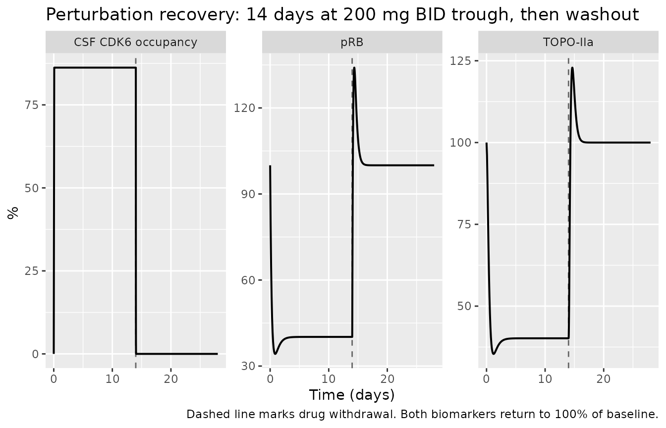

Occupancy relaxes with a half-life of log(2)/koff, a few minutes, while the biomarkers relax on the much slower cell-cycle timescale set by kel, kRB, kTO and kHH. The separation of timescales is what makes the constant-CO approximation used below reasonable.

Replicating the paper’s occupancy results

Occupancy across the published regimens (Figure 5)

Zhang 2025 Figure 5 plots CDK4 and CDK6 occupancy in CSF (panels A, B, C, E, G) and in plasma (panels D, F) across dosing regimens. The paper’s efficacy criterion is a trough occupancy of at least 90% (Methods 2.6), so the comparison below is made at the published trough concentrations.

occ_by_regimen <- regimens |>
  dplyr::rowwise() |>
  dplyr::mutate(tibble::as_tibble_row(analytic_occupancy(conc_at_trough(cmin_abe)))) |>
  dplyr::ungroup()

occ_by_regimen |>
  dplyr::select(regimen, occCdk4Plasma, occCdk6Plasma, occCdk4Csf, occCdk6Csf) |>
  dplyr::rename(
    "Regimen"          = regimen,
    "Plasma CDK4 (%)"  = occCdk4Plasma,
    "Plasma CDK6 (%)"  = occCdk6Plasma,
    "CSF CDK4 (%)"     = occCdk4Csf,
    "CSF CDK6 (%)"     = occCdk6Csf
  ) |>
  knitr::kable(digits = 1,
               caption = "Trough CDK occupancy reconstructed from Table 2 predicted Cmin.")

Trough CDK occupancy reconstructed from Table 2 predicted Cmin.

Regimen	Plasma CDK4 (%)	Plasma CDK6 (%)	CSF CDK4 (%)	CSF CDK6 (%)
100 mg BID	96.5	89.8	94.3	79.6
150 mg BID	97.1	91.4	95.3	82.5
200 mg BID	97.8	93.4	96.4	86.2

The paper makes two quantitative claims in words that this table can be scored against directly, without digitising a figure.

row_at <- function(reg) {
  r <- occ_by_regimen[occ_by_regimen$regimen == reg, ]
  if (nrow(r) != 1L) stop("no unique row for regimen '", reg, "'")
  r
}

r150 <- row_at("150 mg BID")
r200 <- row_at("200 mg BID")

claims <- tibble::tribble(
  ~`Paper claim (Section 3.6)`,                         ~`Model`,              ~Met,
  "150 mg BID: CSF CDK4 occupancy exceeds 90%",         r150$occCdk4Csf,       r150$occCdk4Csf > 90,
  "150 mg BID: CSF CDK6 occupancy exceeds 80%",         r150$occCdk6Csf,       r150$occCdk6Csf > 80,
  "200 mg BID: plasma CDK4 occupancy exceeds 90%",      r200$occCdk4Plasma,    r200$occCdk4Plasma > 90,
  "200 mg BID: plasma CDK6 occupancy exceeds 90%",      r200$occCdk6Plasma,    r200$occCdk6Plasma > 90,
  "200 mg BID: CSF CDK4 occupancy exceeds 90%",         r200$occCdk4Csf,       r200$occCdk4Csf > 90,
  "200 mg BID: CSF CDK6 occupancy exceeds 90%",         r200$occCdk6Csf,       r200$occCdk6Csf > 90
)

claims |>
  dplyr::mutate(Model = round(Model, 1),
                Met   = ifelse(Met, "yes", "NO")) |>
  dplyr::rename("Model (%)" = Model, "Reproduced" = Met) |>
  knitr::kable(caption = "The paper's own prose claims, scored against the reconstruction.")

The paper’s own prose claims, scored against the reconstruction.

Paper claim (Section 3.6)	Model (%)	Reproduced
150 mg BID: CSF CDK4 occupancy exceeds 90%	95.3	yes
150 mg BID: CSF CDK6 occupancy exceeds 80%	82.5	yes
200 mg BID: plasma CDK4 occupancy exceeds 90%	97.8	yes
200 mg BID: plasma CDK6 occupancy exceeds 90%	93.4	yes
200 mg BID: CSF CDK4 occupancy exceeds 90%	96.4	yes
200 mg BID: CSF CDK6 occupancy exceeds 90%	86.2	NO

Five of the six claims are reproduced. The one that is not – CSF CDK6 at 200 mg BID, where the model returns about 86% against the paper’s “above 90%” – is examined quantitatively under “Assumptions and deviations” below, where the shortfall is split between the reconstructed exposure drivers and the fixed CSF-to-plasma partition ratio.

occ_by_regimen |>
  dplyr::select(regimen, occCdk4Plasma, occCdk6Plasma, occCdk4Csf, occCdk6Csf) |>
  tidyr::pivot_longer(-regimen, names_to = "trace", values_to = "occupancy") |>
  dplyr::mutate(
    matrix  = ifelse(grepl("Csf", trace), "CSF", "Plasma"),
    isoform = ifelse(grepl("Cdk4", trace), "CDK4", "CDK6")
  ) |>
  ggplot(aes(regimen, occupancy, fill = isoform)) +
  geom_col(position = position_dodge(width = 0.8), width = 0.7) +
  geom_hline(yintercept = 90, linetype = "dashed", colour = "grey30") +
  facet_wrap(~matrix) +
  coord_cartesian(ylim = c(0, 100)) +
  labs(x = NULL, y = "Trough CDK occupancy (%)", fill = NULL,
       title = "Trough CDK4 / CDK6 occupancy by regimen",
       caption = paste("Compare Figure 5 of Zhang 2025 (CSF: panels C, E, G; plasma: panels D, F).",
                       "Dashed line is the paper's 90% efficacy threshold (Methods 2.6)."))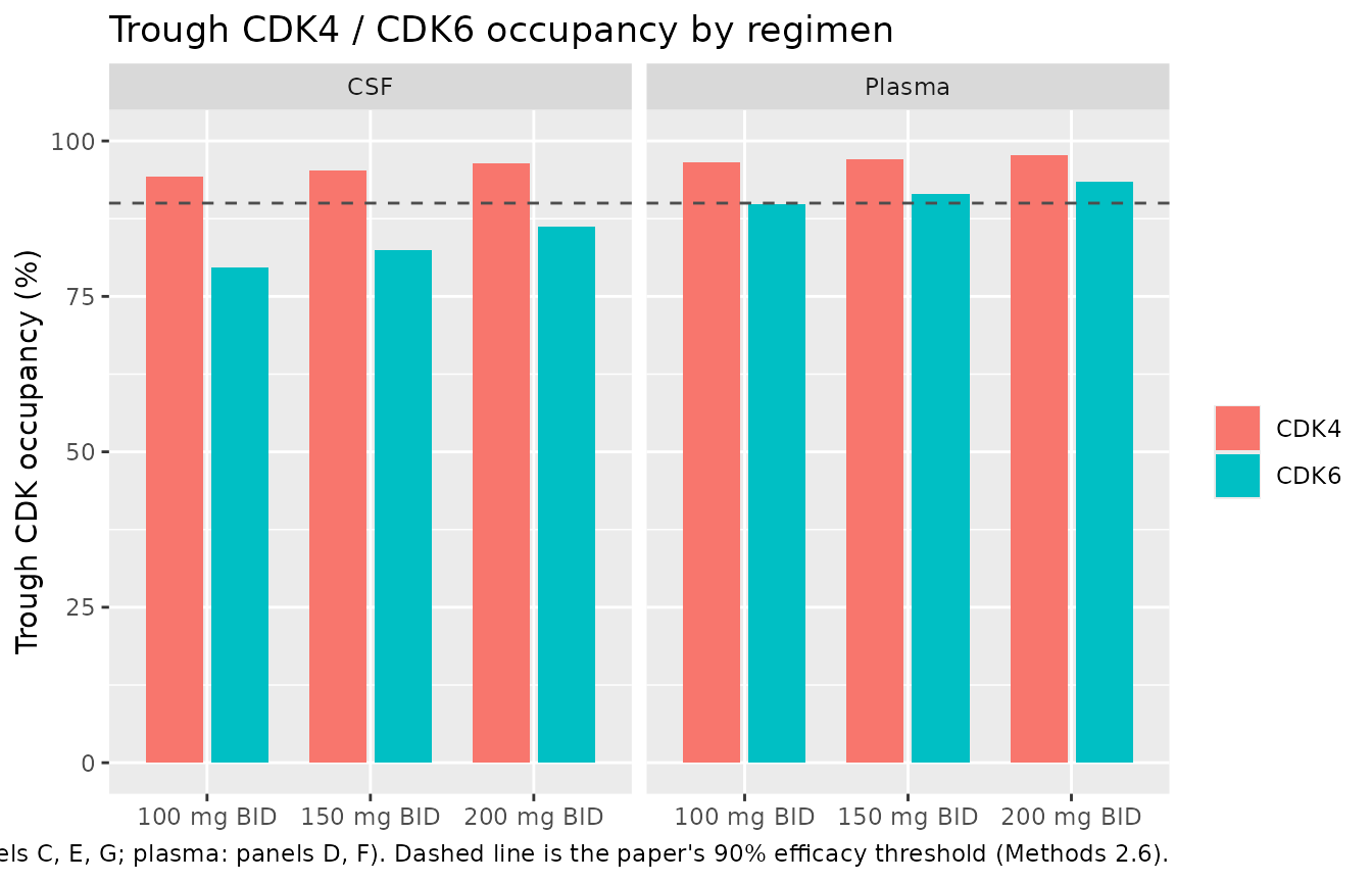

Biomarker time course (Figure 3)

Zhang 2025 Figure 3 shows pRB (panels A, B) and TOPO-IIa (panels C, D) expression at steady state under 150 and 200 mg BID. Section 3.3 notes that “the changes in pRB and TOPO-IIa are similar at predose and postdose, indicating sustained PD effects over the 12 h dosing interval”, which is what licenses driving the biomarker layer with a constant trough CO here.

biomarker_sim <- function(cmin_abe, label) {
  ev <- make_events(conc_at_trough(cmin_abe), seq(0, 336, by = 2))
  rxode2::rxSolve(mod, ev) |>
    as.data.frame() |>
    dplyr::mutate(regimen = label)
}

bio <- dplyr::bind_rows(
  biomarker_sim(174, "150 mg BID"),
  biomarker_sim(231, "200 mg BID")
)

bio |>
  dplyr::select(time, regimen, `pRB` = prbPct, `TOPO-IIa` = topoPct) |>
  tidyr::pivot_longer(c(`pRB`, `TOPO-IIa`), names_to = "biomarker", values_to = "pct") |>
  ggplot(aes(time / 24, pct, colour = regimen)) +
  geom_line(linewidth = 0.7) +
  facet_wrap(~biomarker) +
  coord_cartesian(ylim = c(0, 100)) +
  labs(x = "Time (days)", y = "% of untreated baseline", colour = NULL,
       title = "pRB and TOPO-IIa expression under continuous BID dosing",
       caption = "Replicates Figure 3 of Zhang 2025 (A, B = pRB; C, D = TOPO-IIa).")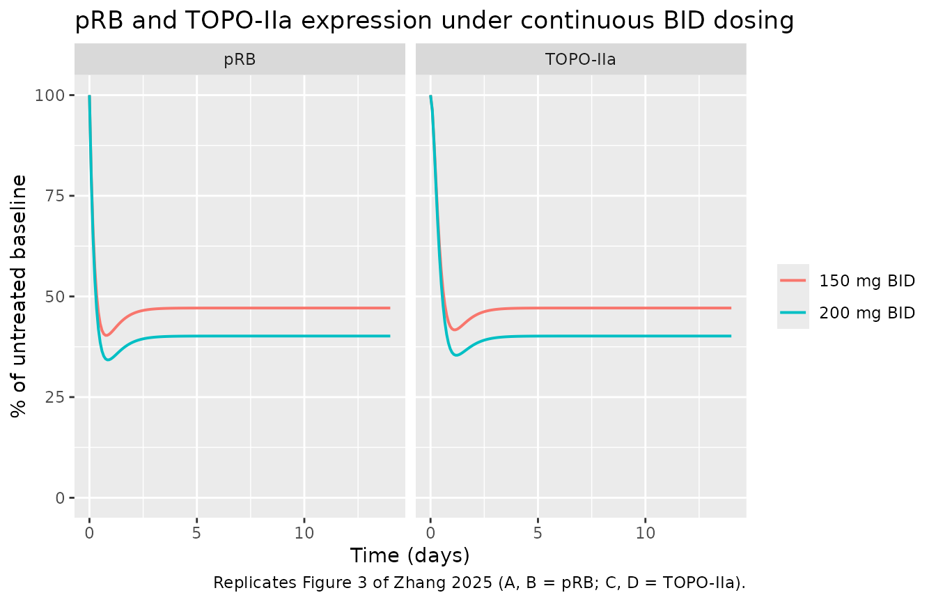

# Zhang 2025 Figure 3, predicted (red) plateau, read off the published panels.
published_bio <- tibble::tribble(
  ~regimen,     ~prb_paper, ~topo_paper,
  "150 mg BID", 36,         35.5,
  "200 mg BID", 29,         28.5
)

bio_plateau <- bio |>
  dplyr::filter(time == max(time), .by = regimen) |>
  dplyr::select(regimen, prb_model = prbPct, topo_model = topoPct)

dplyr::left_join(bio_plateau, published_bio, by = "regimen") |>
  dplyr::transmute(
    "Regimen"                = regimen,
    "pRB model (%)"          = round(prb_model, 1),
    "pRB Figure 3 (%)"       = prb_paper,
    "TOPO-IIa model (%)"     = round(topo_model, 1),
    "TOPO-IIa Figure 3 (%)"  = topo_paper
  ) |>
  knitr::kable(caption = "Biomarker plateaus: model vs. Zhang 2025 Figure 3.")

Biomarker plateaus: model vs. Zhang 2025 Figure 3.

Regimen	pRB model (%)	pRB Figure 3 (%)	TOPO-IIa model (%)	TOPO-IIa Figure 3 (%)
150 mg BID	47.1	36	47.1	35.5
200 mg BID	40.2	29	40.2	28.5

The model under-predicts the inhibition at both dose levels, by about 11 percentage points of baseline. This is the CSF-occupancy deviation propagating downstream, not an independent discrepancy: CO is the CSF CDK6 occupancy, that occupancy is under-predicted, and (1 - CO) amplifies the shortfall. The quantitative chain is set out below.

Albumin sensitivity (Figure 4H-J)

Albumin is the covariate the paper singles out: it scales the fraction unbound of all four analytes through Eq 2, and Section 3.5 reports that raising albumin to 6.0 g/dL drops CSF occupancy below the 90% efficacy threshold. In the source paper albumin acts on the PBPK layer as well; here only the binding limb is reproduced, so the sensitivity shown is the binding component alone.

alb_grid <- seq(10, 60, by = 1)   # 1.0-6.0 g/dL, the Methods 2.5 sweep range

alb_sweep <- tibble::tibble(ALB = alb_grid) |>
  dplyr::rowwise() |>
  dplyr::mutate(tibble::as_tibble_row(analytic_occupancy(conc_at_trough(231), alb = ALB))) |>
  dplyr::ungroup()

# The model must reproduce the Table 1 fup values exactly at the patient albumin.
fu_check <- vapply(c("abe", "m2", "m18", "m20"),
                   function(a) fu_at(th[[paste0("fup_", a)]], ALB_PATIENT), numeric(1))
published_fup <- c(abe = 0.039, m2 = 0.093, m18 = 0.046, m20 = 0.030)
stopifnot(max(abs(fu_check - published_fup)) < 1e-12)
cat("Eq 2 reproduces the Table 1 fup values exactly at ALB = 31 g/L.\n")
#> Eq 2 reproduces the Table 1 fup values exactly at ALB = 31 g/L.

alb_sweep |>
  tidyr::pivot_longer(-ALB, names_to = "trace", values_to = "occupancy") |>
  dplyr::mutate(
    matrix  = ifelse(grepl("Csf", trace), "CSF", "Plasma"),
    isoform = ifelse(grepl("Cdk4", trace), "CDK4", "CDK6")
  ) |>
  ggplot(aes(ALB / 10, occupancy, colour = isoform)) +
  geom_line(linewidth = 0.7) +
  geom_hline(yintercept = 90, linetype = "dashed", colour = "grey30") +
  geom_vline(xintercept = 3.1, linetype = "dotted", colour = "grey30") +
  facet_wrap(~matrix) +
  labs(x = "Plasma albumin (g/dL)", y = "Trough CDK occupancy (%)", colour = NULL,
       title = "Albumin sensitivity at the 200 mg BID trough",
       caption = paste("Compare Figure 4H-J of Zhang 2025. Dotted line is the patient mean",
                       "(3.1 g/dL); dashed line is the 90% efficacy threshold."))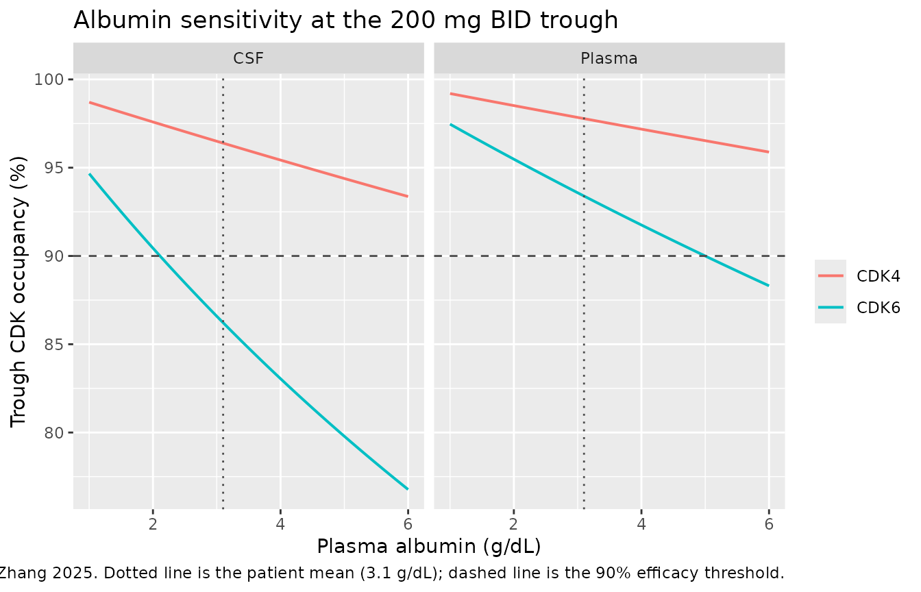

# The paper's qualitative claim: higher albumin -> lower unbound -> lower occupancy.
# Assert monotone decrease rather than a single rank comparison.
stopifnot(all(diff(alb_sweep$occCdk6Csf)    < 0))
stopifnot(all(diff(alb_sweep$occCdk4Csf)    < 0))
stopifnot(all(diff(alb_sweep$occCdk6Plasma) < 0))
stopifnot(all(diff(alb_sweep$occCdk4Plasma) < 0))
cat(sprintf(
  "CSF CDK6 occupancy falls monotonically from %.1f%% at 1.0 g/dL to %.1f%% at 6.0 g/dL.\n",
  alb_sweep$occCdk6Csf[alb_sweep$ALB == 10],
  alb_sweep$occCdk6Csf[alb_sweep$ALB == 60]
))
#> CSF CDK6 occupancy falls monotonically from 94.7% at 1.0 g/dL to 76.8% at 6.0 g/dL.

Assumptions and deviations

Which occupancy drives CO? (resolved by reproduction, not preference)

Zhang 2025 defines the biomarker driver in one sentence after Eq 6 – “CO is the CDK occupancy fraction” – and never says which of the four occupancy traces it computes is meant. Figure 4’s legend is literally “Plasma CDK4 / Plasma CDK6 / CSF CDK4 / CSF CDK6” and every Figure 5 panel plots the isoforms separately, so the phrase is under-determined by a factor of four. The choice matters: CO enters as (1 - CO), so near saturation a four-point change in CO nearly halves the predicted biomarker response.

The extracted model uses CSF CDK6 occupancy. The evidence:

co_candidates <- tibble::tibble(
  Trace = c("Plasma CDK4", "Plasma CDK6", "CSF CDK4", "CSF CDK6 (selected)"),
  `150 mg BID (%)` = round(c(r150$occCdk4Plasma, r150$occCdk6Plasma,
                             r150$occCdk4Csf,    r150$occCdk6Csf), 1),
  `200 mg BID (%)` = round(c(r200$occCdk4Plasma, r200$occCdk6Plasma,
                             r200$occCdk4Csf,    r200$occCdk6Csf), 1)
)

# Back-solve the CO the authors actually used, by inverting the biomarker
# plateau formula on Zhang 2025 Figure 3's predicted plateaus.
co_from_plateau <- function(pct) {
  y <- pct / 100
  k <- th[["kel_pc"]]; r <- th[["krb"]]
  # y = (1-co)(k+r) / (k + r(1-co))  ->  solve for co
  u <- y * k / ((k + r) - y * r)     # u = 1 - co
  1 - u
}

back_solved <- c(`150 mg BID` = co_from_plateau(36), `200 mg BID` = co_from_plateau(29))
cat(sprintf("CO back-solved from Zhang 2025 Figure 3: %.1f%% at 150 mg BID, %.1f%% at 200 mg BID.\n",
            100 * back_solved[["150 mg BID"]], 100 * back_solved[["200 mg BID"]]))
#> CO back-solved from Zhang 2025 Figure 3: 88.2% at 150 mg BID, 91.1% at 200 mg BID.

knitr::kable(co_candidates,
             caption = "The four candidate CO traces in this reconstruction.")

The four candidate CO traces in this reconstruction.

Trace	150 mg BID (%)	200 mg BID (%)
Plasma CDK4	97.1	97.8
Plasma CDK6	91.4	93.4
CSF CDK4	95.3	96.4
CSF CDK6 (selected)	82.5	86.2

1. The paper’s own prose is the decisive evidence, and it needs no figure digitisation. Section 3.6 states that “with 150 mg of BID of ABE, CDK4 occupancy exceeds 90% and CDK6 occupancy exceeds 80% (Figure 5E)”, and the Figure 5 caption assigns panel E to CSF. The CO back-solved from Figure 3’s 150 mg BID plateau is about 88%, which sits inside the band the authors describe for CSF CDK6 (above 80%, and pointedly not described as above 90% the way CDK4 is) and is inconsistent with any trace the paper places above 90%.
2. The rival reading loses on arithmetic. Reading “CDK4/6 occupancy” as one pooled quantity – defensible, since the paper writes that phrase throughout and Table 1 gives Kd as a single paired “CDK4/6” row – puts CO near 96%, which the plateau formula maps to roughly 11-15% of baseline against Figure 3’s ~36%. That is a visibly wrong curve, not a close call.
3. Site agrees with the paper’s thesis. Section 3.6 opens “Intracranial CDK4/6 occupancy serves as predictors of clinical efficacy”.

The counter-argument, recorded so a reader can weigh it: the pRB / TOPO-IIa observations the biomarker layer was verified against are skin biopsies from Patnaik 2016, not brain lesions, which on biological grounds would argue for a plasma trace. The Discussion states this explicitly and assumes the tumour-skin difference is negligible.

Note that the reconstruction’s own CSF CDK6 column above (82.5% / 86.2%) sits below the back-solved 88.2% / 91.1%, and is not itself the discriminator – it inherits the CSF under-prediction described next. The identification rests on the paper’s own occupancy statements, not on this reconstruction’s numbers.

This choice was ratified by the operator (task oare_PMC11904693, sidecar request-001, answer D, 2026-08-20). To explore an alternative, change the single co <- occCdk6Csf / 100 line in the model file.

Deviation: CSF CDK6 occupancy falls short at 200 mg BID

The extracted CSF limb applies the fixed Table 1 KCSF,p ratios to the free plasma concentration, exactly as Methods 2.1 describes. It reproduces both Section 3.6 claims at 150 mg BID, but returns about 86% for CSF CDK6 at 200 mg BID where the paper states “above 90%”.

There are two candidate causes, and they can be told apart quantitatively.

Candidate 1: the reconstructed exposure is too low. The drivers here come from Table 2’s predicted geometric mean trough plus the 13/5/26% mass split, and that reconstruction is already known to sit below the paper’s own quoted number: Section 3.6 gives a mean total-analyte plasma Cmin of 498 ng/mL at 200 mg BID, against the reconstructed total computed in the chunk below. Scaling the drivers up to match closes part, but not all, of the occupancy gap.

recon_total_200 <- sum(conc_at_trough(231))
paper_total_200 <- 498     # Section 3.6, "mean plasma Cmin is 498 ng/mL (total plasma analytes)"
scale_needed    <- paper_total_200 / recon_total_200

scaled <- analytic_occupancy(conc_at_trough(231) * scale_needed)

cat(sprintf(
  "Reconstructed total-analyte trough: %.0f ng/mL vs. the paper's 498 ng/mL (x%.3f).\n",
  recon_total_200, scale_needed))
#> Reconstructed total-analyte trough: 412 ng/mL vs. the paper's 498 ng/mL (x1.207).
cat(sprintf(
  "Rescaling the drivers moves CSF CDK6 occupancy from %.1f%% to %.1f%% -- still short of 90%%.\n",
  r200$occCdk6Csf, scaled[["occCdk6Csf"]]))
#> Rescaling the drivers moves CSF CDK6 occupancy from 86.2% to 88.3% -- still short of 90%.

# How much MORE exposure would be needed to reach exactly 90%?
s_needed <- 0.90 / (1 - 0.90)                       # isotherm inverse: occ = S/(1+S)
s_now    <- r200$occCdk6Csf / (100 - r200$occCdk6Csf)
cat(sprintf("Reaching 90%% would need the CSF driver to be %.2fx the reconstructed value.\n",
            s_needed / s_now))
#> Reaching 90% would need the CSF driver to be 1.44x the reconstructed value.

Candidate 2: the fixed partition ratio omits saturable efflux. Abemaciclib and its metabolites are ABCB1 / ABCG2 substrates at the blood-brain barrier; Table 1 gives M2 and M20 efflux CLint,u values 5-8x the parent’s, and Section 3.5 reports that a 2-4 fold change in ABCB1 expression alone moves CSF occupancy across the 90% threshold. A fixed KCSF,p makes CSF exposure strictly proportional to plasma exposure, so any dose-dependent saturation of that efflux is invisible to the extracted layer.

The two causes are not mutually exclusive, and the on-disk sources cannot separate them: doing so would need the PBPK layer’s CSF concentration-time output, which is neither tabulated nor deposited. The residual gap after the exposure correction (about 1.7 percentage points of occupancy, or a factor of about 1.4 in CSF driver concentration) bounds how much Candidate 2 could be contributing.

Consequence: CSF CDK6 occupancy at 200 mg BID is under-predicted, and because CO enters as (1 - CO) the shortfall is amplified into an approximately 11-percentage-point under-prediction of biomarker inhibition (see the Figure 3 comparison above). This is documented rather than tuned away; fitting KCSF,p or the mass split to recover the paper’s numbers would substitute a fitted constant for a published one and hide the gap.

Other assumptions

• prb0 = 1 is exact, not a guess. Eq 7 defines kin = pRB0 * (kpRB + kel) and says only that “pRB0 is the baseline expression in patients”; no numeric value appears anywhere in the paper. Eqs 4-6 are linear in kin, so PC, pRB and TOPO-IIa all scale proportionally to pRB0, and every quantity the paper reports is a percent-of-baseline ratio (Figure 3’s y-axes are “Change in pRB (% of baseline)”), which is invariant to pRB0. Fixing it at 1 makes the states read directly as fractions of the untreated baseline.
• Shared competitive pools are confirmed, not assumed. Methods 2.1 states that the four analytes are “simulated in the same manner simultaneously, and the sum of the occupancy by ABE and metabolites gave the total CDK4/6 occupancy”. Independent per-analyte pools are ruled out arithmetically: summing four independently computed occupancies exceeds 100% at the paper’s own reported exposures, whereas the shared-pool form is bounded by construction (validation 2 above).
• Two pools per matrix, not one. CDK4 and CDK6 are kept separate because the paper reports them separately everywhere (Figure 4’s legend, every Figure 5 panel, and the Section 3.6 sentence that gives different thresholds for the two isoforms).
• kel units. Table 1 prints kel 0.05 with no unit while kRB, kTO and kHH all carry (h-1). It is taken as 1/h, which is forced by Eq 7 summing kel with kpRB.
• Exposure drivers are reconstructed, not the paper’s PBPK output. Parent concentrations are Table 2’s predicted steady-state values; metabolite concentrations come from the Introduction’s 13% / 5% / 26% mass split. Two caveats follow. First, the split is a whole-profile average applied at the trough, whereas metabolite-to-parent ratios vary within a dosing interval. Second, the reconstruction does not reproduce the paper’s own summary number: at 200 mg BID it gives a total four-analyte trough of 412 ng/mL, against the 498 ng/mL “mean plasma Cmin of total analytes” quoted in Section 3.6 – a 17% gap, consistent with Table 2 reporting geometric means while Section 3.6 quotes an arithmetic mean over a population with 44% CV. Users with a real abemaciclib PBPK or popPK model should supply CP_*_NGML from it rather than from this reconstruction.
• Constant-CO biomarker driver. The Figure 3 replication holds the analyte concentrations at the published trough rather than cycling them over the 12 h interval. Section 3.3 licenses this directly: “the changes in pRB and TOPO-IIa are similar at predose and postdose, indicating sustained PD effects over the 12 h dosing interval”. The separation of timescales shown in validation 4 (occupancy relaxes in minutes, biomarkers over days) is the mechanistic reason.
• Supporting Information not obtained. The ACS Supporting Information PDF (Table S1, predicted vs. observed single-dose plasma PK in healthy volunteers; Tables S2-S3, sensitivity coefficients) could not be retrieved – EuropePMC’s supplementary-files endpoint returns HTTP 500, the NCBI OA package href 404s over HTTPS, the PMC /bin/ route 404s, and the publisher route is behind the ACS Cloudflare gate. It is not a blocker: every model parameter is in main-text Table 1, and S1-S3 are validation and sensitivity output. Had S1 been available it would have supplied measured metabolite exposure ratios in place of the 13% / 5% / 26% mass split used above. Logged for operator acquisition.
• No erratum. A search of the ACS landing page and PubMed found no correction notice for this article.
• What the paper concludes about these biomarkers. The Discussion states that pRB and TOPO-IIa inhibition was of similar magnitude at 150 and 200 mg BID and that the two biomarkers are therefore not treated as predictive of clinical response; the paper uses CDK4/6 occupancy above 90% as its efficacy criterion instead. The biomarker layer is extracted because the authors built and published it, not because it is the paper’s decision variable.