Amoxicillin (Mukap 2025)
Source:vignettes/articles/Mukap_2025_amoxicillin.Rmd
Mukap_2025_amoxicillin.RmdModel and source
- Citation: Mukap M, Sprod C, Yoo O, Tefuarani N, Vince J, Laman M, Page-Sharp M, Moore BR, Batty KT, Davis TME, Salman S, Manning L. A simplified amoxicillin regimen with dose frequency based on post-natal age in neonates with confirmed or suspected infection. Antimicrob Agents Chemother. 2025;69(4):e01491-24. doi:10.1128/aac.01491-24.
- Description: Two-compartment population PK model for intravenous amoxicillin in neonates with confirmed or suspected sepsis in Papua New Guinea (Mukap 2025), fitted to dried-blood-spot (DBS) concentrations with an estimated plasma-to-DBS ratio for venous plasma samples. Allometric scaling on body weight (reference 2.8 kg; exponents fixed at 0.75 on CL and Q and 1 on Vc and Vp), exponential maturation of CL with postmenstrual age (centred on 39 weeks) and a 57% step increase in CL for postnatal age above 2 days. Interindividual variability on CL, Vc and the plasma-to-DBS ratio, interoccasion variability on CL and Vc with each dose an occasion, and additive residual error on the log scale for DBS and plasma.
- Article: https://doi.org/10.1128/aac.01491-24
Mukap 2025 characterised intravenous amoxicillin in neonates treated for confirmed or suspected sepsis at Port Moresby General Hospital, Papua New Guinea, and used the model to compare existing and simplified dosing regimens for the probability of target attainment (fT > MIC) and for the proportion of neonates with concentrations above 140 mg/L, the neurotoxicity surrogate.
The structural model was fitted to dried-blood-spot (DBS) concentrations from heel-prick capillary blood. A single venous plasma sample per neonate entered through an estimated “ratio in plasma to in DBS” (Table 2). The model has two compartments with first-order elimination; body weight scales all clearance and volume terms allometrically (reference 2.8 kg, exponents fixed at 0.75 and 1), clearance matures exponentially with postmenstrual age (PMA) and rises by 57% once postnatal age (PNA) exceeds 2 days (Table 2):
CL = 0.856 * (WT / 2.8)^0.75 * exp(0.0816 * (PMA - 39)) * (1 + 0.57 * [PNA > 2 days])
mod <- readModelDb("Mukap_2025_amoxicillin")
ui <- rxode2::rxode(mod)
#> Warning: some etas defaulted to non-mu referenced, possible parsing error: etaiov_cl_1, etaiov_cl_2, etaiov_cl_3, etaiov_cl_4, etaiov_cl_5, etaiov_cl_6, etaiov_cl_7, etaiov_cl_8, etaiov_cl_9, etaiov_cl_10, etaiov_cl_11, etaiov_cl_12, etaiov_cl_13, etaiov_cl_14, etaiov_cl_15, etaiov_cl_16, etaiov_cl_17, etaiov_cl_18, etaiov_cl_19, etaiov_cl_20, etaiov_cl_21, etaiov_vc_1, etaiov_vc_2, etaiov_vc_3, etaiov_vc_4, etaiov_vc_5, etaiov_vc_6, etaiov_vc_7, etaiov_vc_8, etaiov_vc_9, etaiov_vc_10, etaiov_vc_11, etaiov_vc_12, etaiov_vc_13, etaiov_vc_14, etaiov_vc_15, etaiov_vc_16, etaiov_vc_17, etaiov_vc_18, etaiov_vc_19, etaiov_vc_20, etaiov_vc_21
#> as a work-around try putting the mu-referenced expression on a simple line
rxode2 warns that the interoccasion etas are not mu-referenced; that is expected for occasion-indexed random effects and does not affect simulation.
The model returns two concentrations: Cc, the DBS
concentration (central / vc), and Cc_plasma,
the plasma concentration. As printed in the paper,
Cc_plasma = 0.783 * Cc (with interindividual variability on
the ratio). The paper’s own paired samples point the other way (plasma
higher than DBS); see The
plasma-to-DBS ratio below before using Cc_plasma.
Population
177 neonates aged up to 2 months with bacteriologically confirmed (9.0%) or clinically suspected sepsis were enrolled in a prospective observational study (Mukap 2025 Table 1). Median weight was 2.8 kg (IQR 2.1-3.3, range 0.9-5.5), median gestational age 38 weeks (IQR 37-40, range 28-42), median PNA 0 days (IQR 0-2, range 0-48) and median PMA 273 days (39 weeks; range 196-328 days). 57% of those with recorded sex were male (12 unknown). More than three-quarters were term babies with early-onset sepsis. Amoxicillin was given as 30 mg/kg intravenous slow injections over 3 min, twice daily (BD) for the first 7 days of life and three times daily (TDS) thereafter. DBS samples were collected at baseline and 0.5, 1, 4, 12, 24 and 48 h after the first dose (1,145 retained) and one venous plasma sample at about 24 h (134 retained).
str(ui$population)
#> List of 13
#>  $ species       : chr "human"
#>  $ n_subjects    : int 177
#>  $ n_studies     : int 1
#>  $ age_range     : chr "Postnatal age 0-48 days (median 0, IQR 0-2 days)"
#>  $ weight_range  : chr "0.9-5.5 kg (median 2.8, IQR 2.1-3.3 kg)"
#>  $ ga_range      : chr "28-42 weeks (median 38, IQR 37-40)"
#>  $ pma_range     : chr "196-328 days, i.e. 28-47 weeks (median 273 days)"
#>  $ sex_female_pct: num 43
#>  $ race_ethnicity: chr "Papua New Guinean neonates (not further reported)."
#>  $ disease_state : chr "Neonates (<= 2 months) with bacteriologically confirmed (9.0%) or clinically suspected sepsis; 61.0% clinically"| __truncated__
#>  $ dose_range    : chr "30 mg/kg intravenous amoxicillin as a 3-min slow injection (median 80 mg, range 15-96 mg; 9.4-59 mg/kg), twice "| __truncated__
#>  $ regions       : chr "Papua New Guinea (Port Moresby General Hospital neonatal unit)."
#>  $ notes         : chr "Prospective observational PK study. DBS heel-prick samples at baseline, 0.5, 1, 4, 12, 24 and 48 h after the fi"| __truncated__
Source trace
| Quantity | Value | Source |
|---|---|---|
| CL (per 2.8 kg, PMA 39 weeks, PNA <= 2 days) | 0.856 L/h | Table 2, theta1 |
| Vc (per 2.8 kg) | 4.11 L | Table 2, VC |
| Q (per 2.8 kg) | 0.406 L/h | Table 2, Q |
| Vp (per 2.8 kg) | 1.35 L | Table 2, VP |
| Plasma-to-DBS ratio | 0.783 | Table 2, ‘Ratio in plasma to in DBS’ |
| Allometric exponents (CL and Q; Vc and Vp) | 0.75; 1 (fixed) | Supplement section 2 |
| PMA maturation, FMAT = exp(theta (PMA - 39)) | theta = 0.0816 /week | Table 2 |
| PNA effect, CL x (1 + theta) when PNA > 2 days | theta = 0.57 | Table 2 |
| IIV CL, Vc, ratio | 49.5%, 42.2%, 47.7% | Table 2 (100 x sqrt(variance), footnote) |
| IOV CL, Vc (each dose an occasion) | 31.8%, 34.6% | Table 2; Supplement section 2 |
| Residual error, log DBS | 0.182 (log-scale SD) | Table 2, AddLnDBS |
| Residual error, log plasma | 0.584 (log-scale SD) | Table 2 row ‘PropPlasma’, footnote ‘AddLnPlasma’ |
| Two-compartment structure, first-order elimination | – | Results, Pharmacokinetic modeling |
| Plasma = ratio x DBS | – | Methods, Simulations (‘adjusted … by multiplication’) |
Typical-value checks
The Discussion quotes the point clearance estimate as 0.31 L/h/kg, which is theta1 per 2.8 kg (0.856 / 2.8 = 0.306 L/h/kg) for a neonate at PMA 39 weeks and PNA up to 2 days.
The typical DBS profile after a single 30 mg/kg dose in a 2.8 kg neonate at PMA 39 weeks and PNA 0 days is compared with the observed median of the prediction-corrected VPC (Supplementary Figure S4, digitised by the maintainers on the natural-log scale: about 2.85 at 0.5 h, 1.9 at 4 h and 1.0 at 12 h after the dose).
mod_typ <- rxode2::zeroRe(ui)
#> Warning: some etas defaulted to non-mu referenced, possible parsing error: etaiov_cl_1, etaiov_cl_2, etaiov_cl_3, etaiov_cl_4, etaiov_cl_5, etaiov_cl_6, etaiov_cl_7, etaiov_cl_8, etaiov_cl_9, etaiov_cl_10, etaiov_cl_11, etaiov_cl_12, etaiov_cl_13, etaiov_cl_14, etaiov_cl_15, etaiov_cl_16, etaiov_cl_17, etaiov_cl_18, etaiov_cl_19, etaiov_cl_20, etaiov_cl_21, etaiov_vc_1, etaiov_vc_2, etaiov_vc_3, etaiov_vc_4, etaiov_vc_5, etaiov_vc_6, etaiov_vc_7, etaiov_vc_8, etaiov_vc_9, etaiov_vc_10, etaiov_vc_11, etaiov_vc_12, etaiov_vc_13, etaiov_vc_14, etaiov_vc_15, etaiov_vc_16, etaiov_vc_17, etaiov_vc_18, etaiov_vc_19, etaiov_vc_20, etaiov_vc_21
#> as a work-around try putting the mu-referenced expression on a simple line
ev_typ <- data.frame(
  id = 1L,
  time = c(0, seq(0.25, 12, by = 0.25)),
  evid = c(1L, rep(0L, 48)),
  amt = c(30 * 2.8, rep(0, 48)),
  cmt = "central",
  dvid = c(NA_integer_, rep(1L, 48)),
  WT = 2.8, PAGE = 39, PNA = 0, OCC = 1
)
typ <- as.data.frame(rxode2::rxSolve(mod_typ, ev_typ, useLinCmt = FALSE))
#> ℹ omega/sigma items treated as zero: 'etalcl', 'etalvc', 'etalratio_plasma_central', 'etaiov_cl_1', 'etaiov_cl_2', 'etaiov_cl_3', 'etaiov_cl_4', 'etaiov_cl_5', 'etaiov_cl_6', 'etaiov_cl_7', 'etaiov_cl_8', 'etaiov_cl_9', 'etaiov_cl_10', 'etaiov_cl_11', 'etaiov_cl_12', 'etaiov_cl_13', 'etaiov_cl_14', 'etaiov_cl_15', 'etaiov_cl_16', 'etaiov_cl_17', 'etaiov_cl_18', 'etaiov_cl_19', 'etaiov_cl_20', 'etaiov_cl_21', 'etaiov_vc_1', 'etaiov_vc_2', 'etaiov_vc_3', 'etaiov_vc_4', 'etaiov_vc_5', 'etaiov_vc_6', 'etaiov_vc_7', 'etaiov_vc_8', 'etaiov_vc_9', 'etaiov_vc_10', 'etaiov_vc_11', 'etaiov_vc_12', 'etaiov_vc_13', 'etaiov_vc_14', 'etaiov_vc_15', 'etaiov_vc_16', 'etaiov_vc_17', 'etaiov_vc_18', 'etaiov_vc_19', 'etaiov_vc_20', 'etaiov_vc_21'

vpc_median <- data.frame(time = c(0.5, 4, 12), obs_log = c(2.85, 1.9, 1.0)) |>
  mutate(obs_median = exp(obs_log))
typ_check <- vpc_median |>
  left_join(typ |> select(time, Cc), by = "time") |>
  mutate(ratio = Cc / obs_median)
knitr::kable(
  typ_check |>
    select(time, obs_median, Cc, ratio) |>
    rename(
      "Time after dose (h)" = time,
      "Observed VPC median (mg/L)" = obs_median,
      "Typical DBS prediction (mg/L)" = Cc,
      "Predicted / observed" = ratio
    ),
  digits = 2
)| Time after dose (h) | Observed VPC median (mg/L) | Typical DBS prediction (mg/L) | Predicted / observed |
|---|---|---|---|
| 0.5 | 17.29 | 17.59 | 1.02 |
| 4.0 | 6.69 | 7.48 | 1.12 |
| 12.0 | 2.72 | 2.10 | 0.77 |
ggplot(typ, aes(time, Cc)) +
  geom_line() +
  geom_point(data = vpc_median, aes(time, obs_median), colour = "red", size = 2) +
  scale_y_log10() +
  labs(x = "Time after dose (h)", y = "DBS amoxicillin (mg/L)")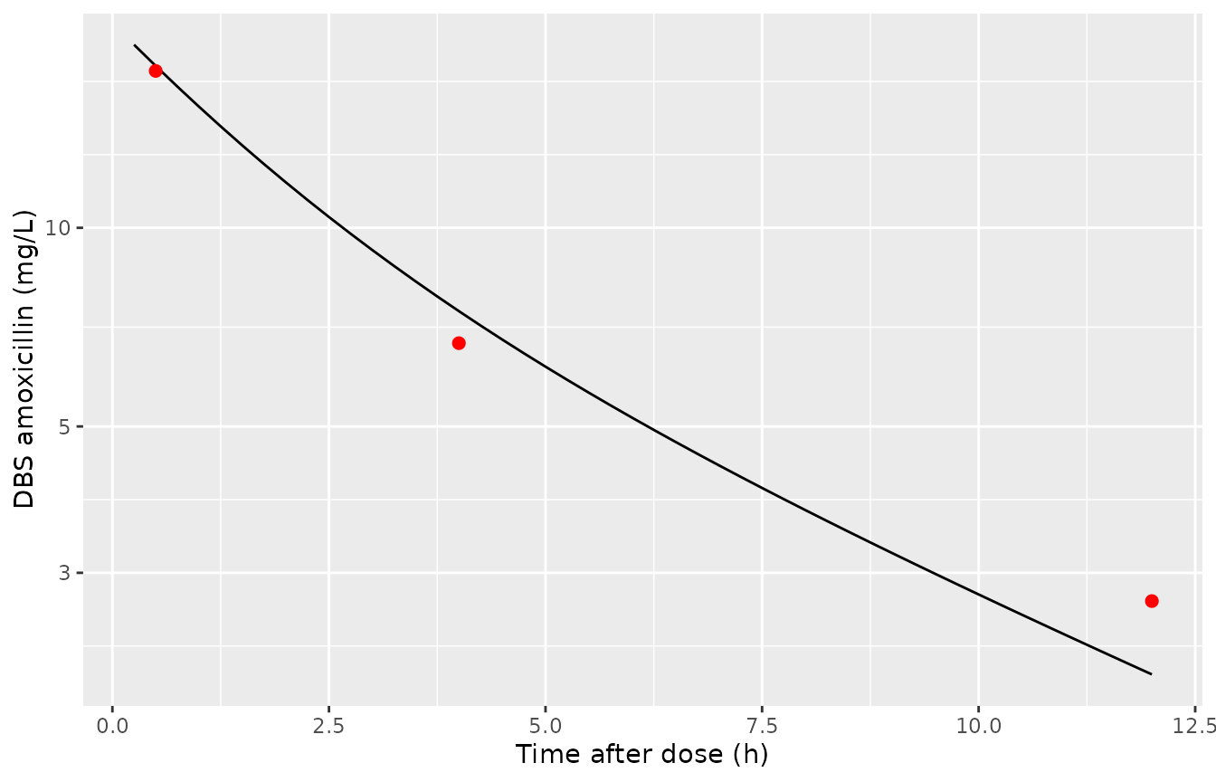
Typical DBS concentration after 30 mg/kg in a 2.8 kg neonate (PMA 39 weeks, PNA 0 days) against the observed VPC medians of Supplementary Figure S4.
The prediction-corrected medians sit close to the typical curve, as expected for a neonate at the cohort median weight and PMA.
Virtual cohort
The paper simulated 1,000 boys and 1,000 girls per PNA band (< 3 days, 3-7 days, > 7 days) and per PMA week from 33 to 41, with weights from preterm weight-for-age data that are not reproduced in the paper. Here a smaller cohort is drawn from the Table 1 marginals instead: PMA normal around 39 weeks (SD 2.15 weeks, matching the 37-40 week IQR; truncated to 28-47) and weight log-normal around 2.8 kg (log-SD 0.335, matching the 2.1-3.3 kg IQR; truncated to 0.9-5.5), correlated at an assumed 0.7. Baseline PNA is half 0-2 days, a quarter 3-7 days and a quarter 8-28 days. PNA (in whole days, as Table 1 reports it) and PMA advance with time on treatment, so the PNA step on clearance and the PNA-based switch in dosing frequency both happen during the simulation.
set.seed(2025)
n_sub <- 200
z1 <- rnorm(n_sub)
z2 <- 0.7 * z1 + sqrt(1 - 0.7^2) * rnorm(n_sub)
cohort <- data.frame(
  id = seq_len(n_sub),
  PMA0 = pmin(pmax(39 + 2.15 * z1, 28), 47),
  WT = pmin(pmax(exp(log(2.8) + 0.335 * z2), 0.9), 5.5),
  PNA0 = sample(c(
    sample(0:2, n_sub / 2, replace = TRUE),
    sample(3:7, n_sub / 4, replace = TRUE),
    sample(8:28, n_sub / 4, replace = TRUE)
  ))
) |>
  mutate(pna_band = cut(PNA0, c(-1, 2, 7, Inf), labels = c("0-2 d", "3-7 d", "> 7 d")))
summary(cohort[, c("PMA0", "WT", "PNA0")])
#>       PMA0             WT             PNA0
#>  Min.   :33.73   Min.   :1.403   Min.   : 0.000
#>  1st Qu.:37.44   1st Qu.:2.221   1st Qu.: 1.000
#>  Median :38.90   Median :2.718   Median : 2.500
#>  Mean   :39.00   Mean   :2.907   Mean   : 6.205
#>  3rd Qu.:40.56   3rd Qu.:3.389   3rd Qu.: 7.250
#>  Max.   :45.13   Max.   :5.500   Max.   :28.000
table(cohort$pna_band)
#>
#> 0-2 d 3-7 d > 7 d
#>   100    50    50
Dosing regimens
The regimens of the paper’s Simulations section and Figure 1. The dosing interval at each dose is chosen from the neonate’s PNA at that time (whole days): BD while PNA is at or below the cut-off, then the later frequency.
regimens <- tibble::tribble(
  ~regimen, ~mgkg, ~cutoff_d, ~tau_late, ~label,
  "png", 30, 7, 6, "PNG: 30 mg/kg BD to day 7, then QID",
  "who", 50, 7, 8, "WHO: 50 mg/kg BD to day 7, then TDS",
  "meningitis", 100, 7, 8, "Meningitis: 100 mg/kg BD to day 7, then TDS",
  "proposed", 30, 2, 8, "Proposed: 30 mg/kg BD to day 2, then TDS",
  "fixed", NA, 2, 8, "Fixed: 52 mg (< 3 kg) or 104 mg, BD to day 2, then TDS"
)
horizon <- 96

dose_times <- function(pna0, cutoff_d, tau_late, horizon) {
  t <- 0
  out <- numeric(0)
  while (t < horizon) {
    out <- c(out, t)
    t <- t + if (floor(pna0 + t / 24) > cutoff_d) tau_late else 12
  }
  out
}

subject_events <- function(s, reg, horizon, obs_step) {
  dt <- dose_times(s$PNA0, reg$cutoff_d, reg$tau_late, horizon)
  amt <- if (is.na(reg$mgkg)) ifelse(s$WT < 3, 52, 104) else reg$mgkg * s$WT
  obs <- sort(unique(c(seq(0, horizon, by = obs_step), dt + 0.05)))
  d <- rbind(
    data.frame(time = dt, evid = 1L, amt = amt, dvid = NA_integer_),
    data.frame(time = obs, evid = 0L, amt = 0, dvid = 1L)
  )
  d <- d[order(d$time, -d$evid), ]
  # Each dose is an occasion; the model encodes 21.
  d$OCC <- pmin(pmax(findInterval(d$time, dt), 1), 21)
  d$id <- s$id
  d$cmt <- "central"
  d$WT <- s$WT
  d$PAGE <- s$PMA0 + d$time / 168
  # PNA in whole days, converted to months.
  d$PNA <- floor(s$PNA0 + d$time / 24) / 30.4375
  d
}

build_events <- function(cohort, reg, horizon, obs_step = 0.25) {
  do.call(rbind, lapply(
    split(cohort, cohort$id), subject_events,
    reg = reg, horizon = horizon, obs_step = obs_step
  ))
}
Neurotoxicity surrogate: replicating Figure 1 B
Figure 1 B reports the percentage of simulated neonates with plasma
concentrations above 140 mg/L: 6.9% for the existing PNG regimen, 24.9%
for the WHO regimen, 84.5% for 100 mg/kg (text), 6.1% for the proposed
regimen and 4.1% for fixed-volume dosing. The simulation length and
whether residual error was added are not stated; here the maximum
individual prediction over the first 96 h is used. The same subjects
(same random effects) are used for every regimen. Both readings of the
plasma-to-DBS ratio are shown: the packaged Cc_plasma
(plasma = 0.783 x DBS) and the alternative plasma = DBS / 0.783.
sims <- list()
for (k in seq_len(nrow(regimens))) {
  reg <- regimens[k, ]
  ev <- build_events(cohort, reg, horizon)
  rxode2::rxSetSeed(20250304)
  s <- as.data.frame(rxode2::rxSolve(ui, ev, useLinCmt = FALSE, returnType = "data.frame"))
  s$regimen <- reg$regimen
  sims[[reg$regimen]] <- s
}
sim_all <- bind_rows(sims)

cmax_sub <- sim_all |>
  group_by(regimen, id) |>
  summarise(
    cmax_dbs = max(Cc),
    cmax_plasma = max(Cc_plasma),
    cmax_plasma_alt = max(Cc / ratio_plasma_central),
    .groups = "drop"
  )
neuro <- cmax_sub |>
  group_by(regimen) |>
  summarise(
    pct_plasma = 100 * mean(cmax_plasma > 140),
    pct_plasma_alt = 100 * mean(cmax_plasma_alt > 140),
    pct_dbs = 100 * mean(cmax_dbs > 140),
    .groups = "drop"
  ) |>
  left_join(
    data.frame(
      regimen = c("png", "who", "meningitis", "proposed", "fixed"),
      published = c(6.9, 24.9, 84.5, 6.1, 4.1)
    ),
    by = "regimen"
  ) |>
  left_join(regimens |> select(regimen, label), by = "regimen") |>
  arrange(match(regimen, regimens$regimen))

knitr::kable(
  neuro |>
    select(label, published, pct_plasma, pct_plasma_alt, pct_dbs) |>
    rename(
      "Regimen" = label,
      "Published (%)" = published,
      "Cc_plasma = 0.783 x DBS (%)" = pct_plasma,
      "Plasma = DBS / 0.783 (%)" = pct_plasma_alt,
      "DBS (%)" = pct_dbs
    ),
  digits = 1,
  caption = "Percentage of neonates with a maximum concentration above 140 mg/L over 96 h. Replicates Figure 1 B of Mukap 2025."
)| Regimen | Published (%) | Cc_plasma = 0.783 x DBS (%) | Plasma = DBS / 0.783 (%) | DBS (%) |
|---|---|---|---|---|
| PNG: 30 mg/kg BD to day 7, then QID | 6.9 | 0.0 | 7.0 | 0.0 |
| WHO: 50 mg/kg BD to day 7, then TDS | 24.9 | 4.0 | 21.5 | 3.5 |
| Meningitis: 100 mg/kg BD to day 7, then TDS | 84.5 | 26.5 | 62.0 | 45.5 |
| Proposed: 30 mg/kg BD to day 2, then TDS | 6.1 | 0.5 | 7.0 | 0.0 |
| Fixed: 52 mg (< 3 kg) or 104 mg, BD to day 2, then TDS | 4.1 | 0.0 | 5.5 | 0.0 |
# The percentages above are tail counts of 200 subjects and can move by a
# few subjects across rxode2 builds, so the dose ordering is asserted on the
# median maximum concentration instead.
cmax_med <- cmax_sub |>
  group_by(regimen) |>
  summarise(med = median(cmax_plasma), .groups = "drop")
med <- setNames(cmax_med$med, cmax_med$regimen)
stopifnot(
  med[["meningitis"]] > 1.5 * med[["who"]],
  med[["who"]] > 1.3 * med[["png"]]
)
The ordering across regimens is reproduced under both readings. The
magnitudes are not: with the packaged Cc_plasma the
percentages fall well below the published ones, while the alternative
reading (plasma = DBS / 0.783) lands close to the published figures for
the 30 and 50 mg/kg regimens and the fixed-volume regimen. The virtual
cohort is not the paper’s (see above), so this is supporting rather than
conclusive evidence; the next section sets out why the alternative is
the more plausible reading.
The plasma-to-DBS ratio
Table 2 labels the estimate 0.783 the “Ratio in plasma to in DBS”, and the Methods (Simulations) state that “the simulated DBS concentrations were then adjusted to free plasma concentrations by multiplication”, i.e. plasma = 0.783 x DBS. That is the relationship the packaged model encodes.
The paper’s own data contradict that direction. In the 135 paired samples, “the amoxicillin concentration ratios between DBS and plasma were 0.48 (95% CI: 0.11-0.97), closely related to the average haematocrit value of 0.49” (Results). DBS was lower than plasma in essentially every pair, as expected for a drug that stays in plasma (DBS approximates whole blood, roughly plasma x (1 - haematocrit)). A ratio fitted to those data as plasma = ratio x DBS would have to be above 1. The data-consistent reading of 0.783 is DBS = 0.783 x plasma, i.e. plasma = DBS / 0.783 = 1.28 x DBS. The neurotoxicity comparison above points the same way.
typ |>
  mutate(plasma_alt = Cc / 0.783) |>
  select(time, Cc, Cc_plasma, plasma_alt) |>
  pivot_longer(-time, names_to = "output", values_to = "conc") |>
  mutate(output = recode(output,
    Cc = "DBS (Cc)",
    Cc_plasma = "Plasma, packaged (0.783 x DBS)",
    plasma_alt = "Plasma, alternative (DBS / 0.783)"
  )) |>
  ggplot(aes(time, conc, colour = output)) +
  geom_line() +
  scale_y_log10() +
  labs(x = "Time after dose (h)", y = "Amoxicillin (mg/L)", colour = NULL) +
  theme(legend.position = "bottom")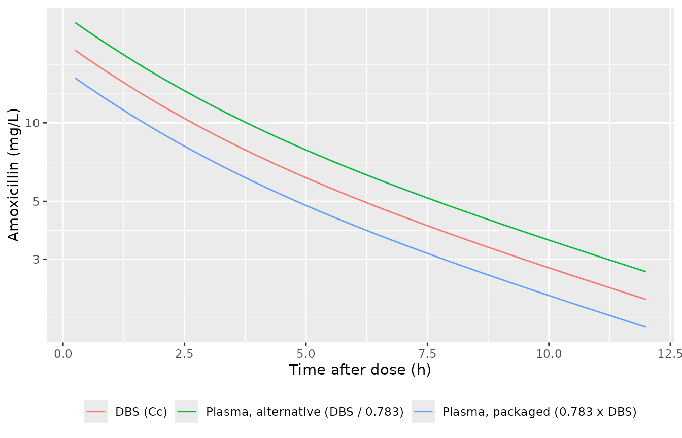
Typical DBS concentration (Cc), the packaged plasma output (Cc_plasma = 0.783 x DBS) and the alternative plasma = DBS / 0.783 after a single 30 mg/kg dose.
To use the alternative reading, take
Cc / ratio_plasma_central from the simulation output
instead of Cc_plasma, as the neurotoxicity chunk above
does. Fixed-effect and DBS predictions are the same under both
readings.
Probability of target attainment in neonates aged 3-7 days
The Results state that the existing PNG regimen gave 94% and 75.1% of neonates aged 3-7 days fT > MIC of at least 70% for MICs of 1 and 4 mg/L, and the proposed regimen 95.6% and 77.4% (Figure 1 C1 and C3). The paper’s 24-hour window is not specified; the second day of treatment (24-48 h) is used here, on a separate cohort of 200 neonates with baseline PNA 3-7 days, with plasma concentrations under both readings.
cohort_37 <- cohort |>
  mutate(id = id, PNA0 = sample(3:7, n_sub, replace = TRUE))
pta_rows <- list()
for (rg in c("png", "proposed")) {
  reg <- regimens[regimens$regimen == rg, ]
  ev <- build_events(cohort_37, reg, horizon = 48, obs_step = 0.1)
  rxode2::rxSetSeed(20250305)
  s <- as.data.frame(rxode2::rxSolve(ui, ev, useLinCmt = FALSE, returnType = "data.frame")) |>
    filter(time >= 24, time <= 48)
  for (mic in c(1, 4)) {
    ft <- s |>
      group_by(id) |>
      summarise(
        ft_plasma = mean(Cc_plasma > mic),
        ft_alt = mean(Cc / ratio_plasma_central > mic),
        .groups = "drop"
      )
    pta_rows[[paste(rg, mic)]] <- data.frame(
      regimen = rg, mic = mic,
      pta_plasma = 100 * mean(ft$ft_plasma >= 0.7),
      pta_alt = 100 * mean(ft$ft_alt >= 0.7)
    )
  }
}
pta <- bind_rows(pta_rows) |>
  left_join(
    data.frame(
      regimen = c("png", "png", "proposed", "proposed"),
      mic = c(1, 4, 1, 4),
      published = c(94, 75.1, 95.6, 77.4)
    ),
    by = c("regimen", "mic")
  )
knitr::kable(
  pta |>
    select(regimen, mic, published, pta_plasma, pta_alt) |>
    rename(
      "Regimen" = regimen,
      "MIC (mg/L)" = mic,
      "Published (%)" = published,
      "Cc_plasma (%)" = pta_plasma,
      "Plasma = DBS / 0.783 (%)" = pta_alt
    ),
  digits = 1,
  caption = "Percentage of neonates aged 3-7 days with fT > MIC of at least 70% on day 2. Compare Figure 1 C1 and C3 of Mukap 2025."
)| Regimen | MIC (mg/L) | Published (%) | Cc_plasma (%) | Plasma = DBS / 0.783 (%) |
|---|---|---|---|---|
| png | 1 | 94.0 | 61.5 | 77.0 |
| png | 4 | 75.1 | 23.0 | 33.5 |
| proposed | 1 | 95.6 | 81.0 | 90.0 |
| proposed | 4 | 77.4 | 39.5 | 55.5 |
stopifnot(
  # Higher MIC can only lower attainment for the same concentrations.
  all(pta$pta_plasma[pta$mic == 4] <= pta$pta_plasma[pta$mic == 1]),
  all(pta$pta_alt[pta$mic == 4] <= pta$pta_alt[pta$mic == 1])
)
The paper’s PTA figures sit higher than both simulated readings for these neonates. Their 24-hour window and cohort (PMA 33-41 weeks across preterm weight-for-age) are not reproducible from the text, so this comparison is qualitative.
Stochastic DBS profiles over the study design
DBS concentrations over the first 48 h under the study regimen (30 mg/kg BD), for the virtual cohort, with the paper’s DBS sampling times marked.
reg_study <- tibble::tibble(regimen = "study", mgkg = 30, cutoff_d = 7, tau_late = 8)
ev_study <- build_events(cohort, reg_study, horizon = 48)
rxode2::rxSetSeed(20250306)
sim_study <- as.data.frame(rxode2::rxSolve(ui, ev_study, useLinCmt = FALSE, returnType = "data.frame"))
sim_study |>
  group_by(time) |>
  summarise(
    p05 = quantile(Cc, 0.05), p50 = median(Cc), p95 = quantile(Cc, 0.95),
    .groups = "drop"
  ) |>
  ggplot(aes(time, p50)) +
  geom_ribbon(aes(ymin = p05, ymax = p95), alpha = 0.25) +
  geom_line() +
  geom_vline(xintercept = c(0.5, 1, 4, 12, 24, 48), linetype = "dotted") +
  scale_y_log10() +
  labs(x = "Time after first dose (h)", y = "DBS amoxicillin (mg/L)")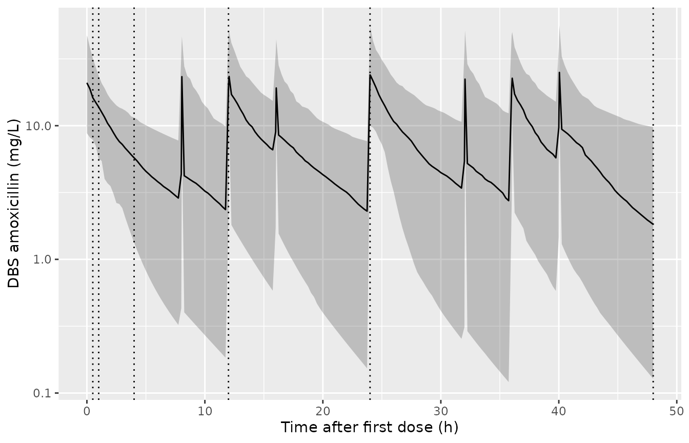
Simulated DBS concentrations (median and 5th-95th percentiles, individual predictions) under 30 mg/kg BD; vertical lines mark the DBS sampling times (0.5, 1, 4, 12, 24, 48 h).
PKNCA validation
Non-compartmental analysis of the simulated DBS concentrations over the first 6 h after the first 30 mg/kg dose (before any second dose in every band), by PNA band. The paper reports no NCA, so there is no published comparison; the check is that the half-life is shorter once the PNA step on clearance applies.
nca_conc <- sim_study |>
  filter(time <= 6, !is.na(Cc)) |>
  select(id, time, Cc) |>
  left_join(cohort |> select(id, pna_band, WT), by = "id") |>
  distinct(id, time, .keep_all = TRUE)
nca_dose <- cohort |>
  transmute(id, pna_band, time = 0, amt = 30 * WT)

conc_obj <- PKNCA::PKNCAconc(nca_conc, Cc ~ time | pna_band + id)
dose_obj <- PKNCA::PKNCAdose(nca_dose, amt ~ time | pna_band + id)
intervals <- data.frame(
  start = 0, end = 6,
  cmax = TRUE, tmax = TRUE, auclast = TRUE, half.life = TRUE
)
nca_res <- PKNCA::pk.nca(PKNCA::PKNCAdata(conc_obj, dose_obj, intervals = intervals))
nca_tab <- as.data.frame(nca_res) |>
  filter(PPTESTCD %in% c("cmax", "auclast", "half.life")) |>
  group_by(pna_band, PPTESTCD) |>
  summarise(median = median(PPORRES, na.rm = TRUE), .groups = "drop") |>
  pivot_wider(names_from = PPTESTCD, values_from = median)
knitr::kable(
  nca_tab |>
    rename(
      "PNA band" = pna_band,
      "Cmax (mg/L)" = cmax,
      "AUC0-6 (mg h/L)" = auclast,
      "t1/2 (h)" = half.life
    ),
  digits = 2,
  caption = "Median DBS NCA after the first 30 mg/kg dose, by PNA band."
)| PNA band | AUC0-6 (mg h/L) | Cmax (mg/L) | t1/2 (h) |
|---|---|---|---|
| 0-2 d | 59.52 | 20.57 | 4.17 |
| 3-7 d | 48.24 | 23.58 | 2.68 |
| > 7 d | 44.16 | 18.46 | 2.94 |
# The PNA step on clearance shortens the half-life in neonates older than
# 2 days; a mis-coded PNA unit or threshold would flatten this contrast.
hl <- setNames(nca_tab$half.life, as.character(nca_tab$pna_band))
stopifnot(hl[["3-7 d"]] < hl[["0-2 d"]])
Assumptions and deviations
-
Plasma-to-DBS ratio direction.
Cc_plasma = ratio x Ccfollows the Table 2 label and the Methods wording. The paper’s paired samples (DBS / plasma 0.48) and haematocrit physiology indicate DBS = ratio x plasma instead, and that reading reproduces the published neurotoxicity percentages much more closely (see above). The maintainers kept the printed relationship;Cc / ratio_plasma_centralgives the alternative. - PNA threshold. The Table 2 equation (CL x 1.57 for PNA > 2 days) is encoded; the Results prose says “> 3 days old”. PNA is supplied in months (register convention) and compared against 2 / 30.4375 months.
- PNA coefficient. The point estimate 0.57 is encoded. The bootstrap median in Table 2, 0.254 (95% CI 0.192-0.379), excludes it; the paper does not comment.
-
Residual error. Both residual errors are additive
on the log scale (
lnorm), per the Supplement (“additive error for the log-transformed data”) and the Table 2 footnote, which defines AddLnPlasma although the table row reads PropPlasma. - Variability scale. Table 2 reports variability as 100 x sqrt(variance); variances are the squared fractions.
-
Interoccasion variability. Each dose is an occasion
(Supplement). The number of occasions is not reported; 21 are encoded (7
days of 8-hourly dosing), all sharing one variance per parameter.
Records with
OCCoutside 1-21 carry no IOV. - Interindividual variability on the ratio is assumed log-normal (exponential), like the other random effects.
-
PMA units. PMA is carried in weeks
(
PAGE, declared in weeks for this model) because the maturation term is centred on 39 weeks. - Virtual cohort. Drawn from the Table 1 marginals with an assumed weight-PMA correlation of 0.7, not from the paper’s PMA-week by PNA-band grid with preterm weight-for-age data. Simulation length (96 h), the use of individual predictions without residual error, and the 24-48 h PTA window are the maintainers’ choices; the paper does not state them.