Propofol and remifentanil haemodynamics (Garraza-Obaldia 2024)
Source:vignettes/articles/GarrazaObaldia_2024_propofol_remifentanil.Rmd
GarrazaObaldia_2024_propofol_remifentanil.RmdModel and source
- Citation: Garraza-Obaldia M, Jaramillo S, Parra-Guillen ZP, Valencia JF, Gambus PL, Troconiz IF. Pharmacodynamic Model of the Hemodynamic Effects of Propofol and Remifentanil and Their Interaction with Noxious Stimulation. Pharmaceutics. 2024;16(12):1615. doi:10.3390/pharmaceutics16121615.
- Description: Semi-mechanistic turnover PD model of the haemodynamic effects of propofol and remifentanil during general anaesthesia in adult women undergoing gynaecological surgery (Garraza-Obaldia 2024). Mean arterial pressure (MAP) and heart rate (HR) are two coupled indirect-response states: propofol inhibits MAP production (Emax in the predicted plasma propofol concentration), remifentanil inhibits HR production (sigmoid Emax in the predicted plasma remifentanil concentration), relative HR feeds back on MAP production as a power function, and the surgical stimulus (hysteroscopy) transiently raises MAP production with a monoexponentially dissipating effect. The predicted plasma concentrations from the Schnider (propofol) and Minto (remifentanil) target-controlled-infusion models are supplied as time-varying covariates; the model has no PK states.
- Article: https://doi.org/10.3390/pharmaceutics16121615 (open access)
- Supplement: https://www.mdpi.com/article/10.3390/pharmaceutics16121615/s1
Garraza-Obaldia et al. modelled mean arterial pressure (MAP) and heart rate (HR) in women anaesthetised with target-controlled infusions (TCI) of propofol and remifentanil. Both responses are turnover (indirect-response) states:
- propofol inhibits MAP production with an Emax function of its predicted plasma concentration (the Hill coefficient was not different from 1 and was removed);
- remifentanil inhibits HR production with a sigmoid Emax function of its predicted plasma concentration and has no direct effect on MAP;
- HR relative to its baseline feeds back on MAP production as
(HR / HR0)^FBHR; the reverse feedback (MAP on HR) was not supported; - the surgical stimulus (hysteroscopy) multiplies MAP production by
1 + thetaStim * exp(-kStim * (t - tStim))from the start of surgery.
The drug exposures are the plasma concentrations that the TCI pumps
predicted from the Schnider (propofol) and Minto (remifentanil) PK
models; nothing was assayed. The packaged model therefore has no PK
states. The concentrations enter as the time-varying covariates
CP_PROPOFOL_UGML (ug/mL) and
CP_REMIFENTANIL_NGML (ng/mL), and the start of surgery as
the time-fixed covariate T_SURG_START (min). Time is in
minutes.
Population
The analysis used 77 ASA I-II women having outpatient gynaecological surgery at Hospital Clinic de Barcelona; three patients with chronic hypertension were excluded from the 80 enrolled (Results; Table 1). The model was fitted to the 56-patient training group, all of whom had hysteroscopy (mean age 42 years, SD 11; mean weight 62 kg, SD 9; mean BMI 24 kg/m^2, SD 4). The 21-patient test group (other procedures) was used for external validation. Patients were assigned to four step-up / step-down TCI schemes: propofol alone, remifentanil alone, steady propofol with varying remifentanil, and steady remifentanil with varying propofol (Section 2.1; Table S1). MAP was measured non-invasively every minute and HR by continuous ECG. Age, weight, BMI, surgery duration, patient position and stimulus type were screened as covariates and none was retained.
Source trace
| Element | Value in model | Source location |
|---|---|---|
| MAP turnover ODE | d/dt(map) = kin_map (1 - f) (hr/rbase_hr)^fb_hr h_stim - kout_map map |
Equation (1); Figure 2B |
| HR turnover ODE | d/dt(hr) = kin_hr (1 - g) - kout_hr hr |
Equation (2); Figure 2B (MAP feedback on HR dropped, Section 3.1) |
| Production rates | kin = kout * baseline |
Section 2.4 (steady state); derived 10.8 mmHg/min and 8.7 bpm/min in Section 3.1 |
Propofol effect f
|
Emax, no Hill exponent | Equation (3); gamma removed (Section 3.1); Figure 2B |
Remifentanil effect g
|
sigmoid Emax | Equation (4); Figure 2B |
HR feedback p
|
(hr/rbase_hr)^fb_hr |
Equation (5) |
Stimulus h
|
1 + emax_stim exp(-kstim (t - T_SURG_START)), 1
before |
Equation (7); Figure 2B |
lec50_propofol |
log(8.79) ug/mL | Table 2, C50Propo |
logitemax_propofol |
logit(0.88) | Table 2, EmaxPropo; logistic constraint (Section 2.4) |
lec50_remifentanil |
log(4.57) ng/mL | Table 2, C50Remi |
logitemax_remifentanil |
logit(0.69) | Table 2, EmaxRemi,HR |
lhill_remifentanil |
log(1.20) | Table 2, gammaRemi |
lrbase_map |
log(88.2) mmHg | Table 2, MAP0 |
lrbase_hr |
log(70.8) bpm | Table 2, HR0 |
lkout |
log(0.123) 1/min | Table 2, kout (one typical value for MAP and HR, Section 3.1) |
lfb_hr |
log(0.806) | Table 2, FBHR |
lkstim |
log(0.021) 1/min | Table 2, kStim |
lemax_stim |
log(0.284) | Table 2, thetaStim |
etalec50_propofol, etalkout_map block |
0.733137, 0.76, 1.109710 | Table 2: IIV 104.0% and 142.6% CV; covariance 0.76 |
etalec50_remifentanil |
0.730139 | Table 2, IIV C50Remi 103.7% CV |
etalrbase_map |
0.00742009 | Table 2, IIV MAP0 8.63% CV |
etalrbase_hr |
0.0205239 | Table 2, IIV HR0 14.4% CV |
etalkout_hr |
0.991474 | Table 2, IIV kout,HR 130.2% CV |
etalkstim |
fixed(0.693147) | Section 3.1: variance held at the equivalent of a 100% CV |
addSd_map |
5.53 mmHg | Table 2, residual error in MAP |
addSd_hr |
4.30 bpm | Table 2, residual error in HR |
The IIV variances use omega^2 = log(1 + CV^2), the
inverse of the CV definition in the footnote of Table 2
(CV = sqrt(exp(omega^2) - 1)).
Deterministic checks
mod <- readModelDb("GarrazaObaldia_2024_propofol_remifentanil")
ui <- rxode2::rxode(mod)
#> ℹ parameter labels from comments will be replaced by 'label()'
th <- ui$theta
Derived production rates and stimulus half-life
The paper reports the derived production rates and the half-life of the stimulus effect.
derived <- tibble::tibble(
  Quantity = c("kin,MAP (mmHg/min)", "kin,HR (bpm/min)", "Stimulus half-life (min)"),
  Model = c(
    exp(th[["lkout"]]) * exp(th[["lrbase_map"]]),
    exp(th[["lkout"]]) * exp(th[["lrbase_hr"]]),
    log(2) / exp(th[["lkstim"]])
  ),
  Paper = c(10.8, 8.7, 33)
)
knitr::kable(derived, digits = 2, caption = "Derived quantities quoted in Results Sections 3.1 and 3.4 and the Discussion.")| Quantity | Model | Paper |
|---|---|---|
| kin,MAP (mmHg/min) | 10.85 | 10.8 |
| kin,HR (bpm/min) | 8.71 | 8.7 |
| Stimulus half-life (min) | 33.01 | 33.0 |
Steady state under constant concentrations
With constant drug concentrations and no stimulus, both ODEs settle at
HR_ss = HR0 * (1 - g(CRemi))MAP_ss = MAP0 * (1 - f(CPropo)) * (1 - g(CRemi))^FBHR
The typical-value model is solved to 600 min (about 100 half-lives of
kout) over a grid of concentrations and compared with this
closed form.
ss_grid <- tidyr::expand_grid(cp = c(0, 2, 4, 8), cr = c(0, 1, 2, 4)) |>
  mutate(id = row_number())
ss_events <- ss_grid |>
  tidyr::crossing(time = c(0, 600)) |>
  transmute(
    id, time,
    evid = 0, amt = 0,
    CP_PROPOFOL_UGML = cp,
    CP_REMIFENTANIL_NGML = cr,
    T_SURG_START = 1e6
  ) |>
  arrange(id, time)

ss_sim <- rxode2::rxSolve(
  rxode2::zeroRe(ui), ss_events,
  rtol = 1e-10, atol = 1e-12, returnType = "data.frame"
) |>
  filter(time == 600)
#> ℹ omega/sigma items treated as zero: 'etalec50_propofol', 'etalkout_map', 'etalec50_remifentanil', 'etalrbase_map', 'etalrbase_hr', 'etalkout_hr', 'etalkstim'
#> Warning: multi-subject simulation without without 'omega'

emax_p <- plogis(th[["logitemax_propofol"]])
ec50_p <- exp(th[["lec50_propofol"]])
emax_r <- plogis(th[["logitemax_remifentanil"]])
ec50_r <- exp(th[["lec50_remifentanil"]])
hill_r <- exp(th[["lhill_remifentanil"]])
fb <- exp(th[["lfb_hr"]])

ss_check <- ss_grid |>
  mutate(
    f = emax_p * cp / (cp + ec50_p),
    g = emax_r * cr^hill_r / (cr^hill_r + ec50_r^hill_r),
    hr_closed = exp(th[["lrbase_hr"]]) * (1 - g),
    map_closed = exp(th[["lrbase_map"]]) * (1 - f) * (1 - g)^fb
  ) |>
  left_join(select(ss_sim, id, map, hr), by = "id")

ss_check |>
  select(cp, cr, map, map_closed, hr, hr_closed) |>
  dplyr::rename(
    "Propofol (ug/mL)" = cp,
    "Remifentanil (ng/mL)" = cr,
    "MAP solved (mmHg)" = map,
    "MAP closed form (mmHg)" = map_closed,
    "HR solved (bpm)" = hr,
    "HR closed form (bpm)" = hr_closed
  ) |>
knitr::kable(digits = 2, caption = "Typical-value steady state against the closed form.")| Propofol (ug/mL) | Remifentanil (ng/mL) | MAP solved (mmHg) | MAP closed form (mmHg) | HR solved (bpm) | HR closed form (bpm) |
|---|---|---|---|---|---|
| 0 | 0 | 88.20 | 88.20 | 70.80 | 70.80 |
| 0 | 1 | 81.31 | 81.31 | 64.01 | 64.01 |
| 0 | 2 | 74.67 | 74.67 | 57.58 | 57.58 |
| 0 | 4 | 64.83 | 64.83 | 48.32 | 48.32 |
| 2 | 0 | 73.81 | 73.81 | 70.80 | 70.80 |
| 2 | 1 | 68.05 | 68.05 | 64.01 | 64.01 |
| 2 | 2 | 62.49 | 62.49 | 57.58 | 57.58 |
| 2 | 4 | 54.25 | 54.25 | 48.32 | 48.32 |
| 4 | 0 | 63.93 | 63.93 | 70.80 | 70.80 |
| 4 | 1 | 58.94 | 58.94 | 64.01 | 64.01 |
| 4 | 2 | 54.12 | 54.12 | 57.58 | 57.58 |
| 4 | 4 | 46.99 | 46.99 | 48.32 | 48.32 |
| 8 | 0 | 51.22 | 51.22 | 70.80 | 70.80 |
| 8 | 1 | 47.22 | 47.22 | 64.01 | 64.01 |
| 8 | 2 | 43.36 | 43.36 | 57.58 | 57.58 |
| 8 | 4 | 37.65 | 37.65 | 48.32 | 48.32 |
# Same parameters on both sides, so only integration error separates them.
stopifnot(
  nrow(ss_check) == 16,
  max(abs(ss_check$map / ss_check$map_closed - 1)) < 1e-5,
  max(abs(ss_check$hr / ss_check$hr_closed - 1)) < 1e-5
)
Propofol at 4 ug/mL alone lowers the typical MAP by about 28%. Remifentanil lowers MAP only through HR, and the HR feedback exponent below 1 damps that effect.
Replicating Figure 4: risk of hypotension
The paper simulated a 90-min procedure (Figure 1): induction targets until 10 min, maintenance targets until 80 min, then both targets set to zero, with hysteroscopy starting at 20 min. Three schemes paired the two drugs at different effect-site targets:
schemes <- tibble::tibble(
  scheme = 1:3,
  propofol_induction = c(4.0, 4.5, 5.0),
  remifentanil_induction = c(3.0, 2.5, 2.0),
  propofol_maintenance = c(2.5, 3.0, 3.5),
  remifentanil_maintenance = c(2.0, 1.5, 1.0)
)
schemes |>
  dplyr::rename(
    "Scheme" = scheme,
    "Propofol induction (ug/mL)" = propofol_induction,
    "Remifentanil induction (ng/mL)" = remifentanil_induction,
    "Propofol maintenance (ug/mL)" = propofol_maintenance,
    "Remifentanil maintenance (ng/mL)" = remifentanil_maintenance
  ) |>
knitr::kable(caption = "Effect-site targets of the three schemes (Figure 1B).")| Scheme | Propofol induction (ug/mL) | Remifentanil induction (ng/mL) | Propofol maintenance (ug/mL) | Remifentanil maintenance (ng/mL) |
|---|---|---|---|---|
| 1 | 4.0 | 3.0 | 2.5 | 2.0 |
| 2 | 4.5 | 2.5 | 3.0 | 1.5 |
| 3 | 5.0 | 2.0 | 3.5 | 1.0 |
The model is driven by plasma concentrations, which the paper obtained by running the Schnider and Minto TCI algorithms. Neither PK model is in this package, so here the plasma concentration is set equal to the effect-site target (a step function). At a constant target, a TCI pump holds plasma and effect site at the same concentration. The approximation therefore differs from the paper only during the few minutes after each target change. In those minutes a real pump overshoots the plasma concentration on the way up and stops infusing on the way down.
For each scheme 200 virtual patients are simulated (the paper used
1000). Hypotension is defined as in the paper: MAP below 60 mmHg, or a
fall of at least 20% from the individual baseline MAP0. The
probabilities use the individual predicted MAP, without residual
error.
n_per_scheme <- 200
times <- 0:90

fig4_events <- schemes |>
  tidyr::crossing(subject = seq_len(n_per_scheme), time = times) |>
  mutate(
    id = (scheme - 1) * n_per_scheme + subject,
    evid = 0, amt = 0,
    CP_PROPOFOL_UGML = case_when(
      time < 10 ~ propofol_induction,
      time < 80 ~ propofol_maintenance,
      TRUE ~ 0
    ),
    CP_REMIFENTANIL_NGML = case_when(
      time < 10 ~ remifentanil_induction,
      time < 80 ~ remifentanil_maintenance,
      TRUE ~ 0
    ),
    T_SURG_START = 20
  ) |>
  select(id, time, evid, amt, CP_PROPOFOL_UGML, CP_REMIFENTANIL_NGML, T_SURG_START, scheme) |>
  arrange(id, time)

rxode2::rxSetSeed(20241215)
fig4_sim <- rxode2::rxSolve(
  ui, fig4_events,
  covsInterpolation = "locf", keep = "scheme", returnType = "data.frame"
)

risk <- fig4_sim |>
  group_by(scheme, time) |>
  summarise(
    p_below60 = mean(map < 60),
    p_drop20 = mean(map <= 0.8 * rbase_map),
    .groups = "drop"
  )
risk |>
  tidyr::pivot_longer(c(p_below60, p_drop20), names_to = "criterion", values_to = "probability") |>
  mutate(criterion = factor(
    criterion,
    levels = c("p_below60", "p_drop20"),
    labels = c("MAP < 60 mmHg", "20% decrease of MAP from baseline")
  )) |>
  ggplot(aes(time, probability, colour = factor(scheme))) +
  annotate("rect", xmin = 20, xmax = 70, ymin = -Inf, ymax = Inf, alpha = 0.15) +
  geom_line() +
  facet_wrap(~criterion, scales = "free_y") +
  labs(x = "Time (min)", y = "Probability", colour = "Scheme") +
  theme_bw()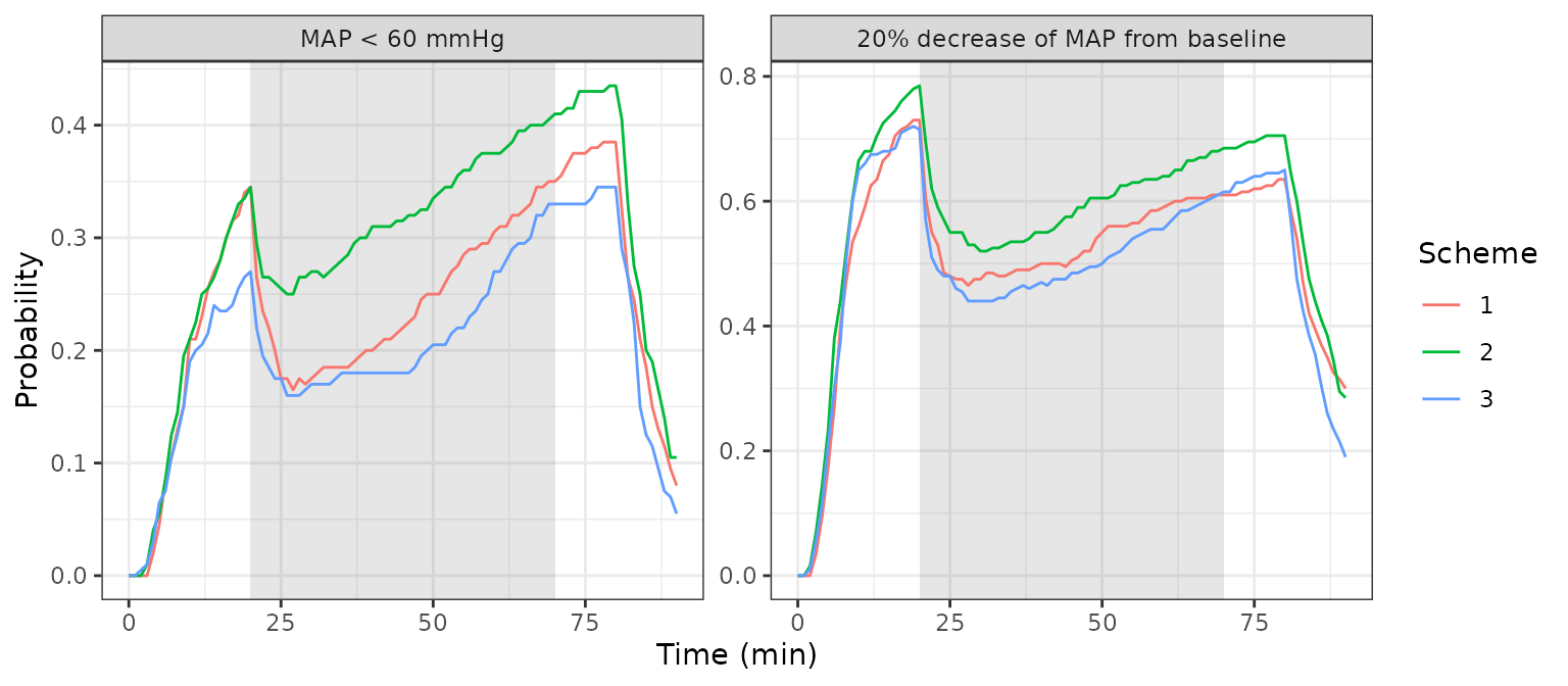
Replicates Figure 4 of Garraza-Obaldia 2024. The grey band is the period of surgery (20-70 min).
The paper reports a maximum probability before surgery of 0.35 (MAP < 60 mmHg) and 0.70 (20% decrease), just before surgery starts, and a maximum during and after surgery of 0.38 and 0.65, at the end of surgery (Results Section 3.4).
pool <- risk |>
  group_by(time) |>
  summarise(p_below60 = mean(p_below60), p_drop20 = mean(p_drop20), .groups = "drop")
at <- function(tm, col) {
  v <- pool[[col]][pool$time == tm]
  if (length(v) != 1L) stop("no unique row at time ", tm)
  v
}
fig4_cmp <- tibble::tibble(
  Quantity = c(
    "P(MAP < 60), 20 min (start of surgery)",
    "P(20% decrease), 20 min (start of surgery)",
    "P(MAP < 60), 80 min (end of infusion)",
    "P(20% decrease), 80 min (end of infusion)"
  ),
  Simulated = c(at(20, "p_below60"), at(20, "p_drop20"), at(80, "p_below60"), at(80, "p_drop20")),
  Paper = c(0.35, 0.70, 0.38, 0.65)
)
knitr::kable(fig4_cmp, digits = 2, caption = "Peak hypotension risk, pooled over the three schemes (600 virtual patients), against Results Section 3.4.")| Quantity | Simulated | Paper |
|---|---|---|
| P(MAP < 60), 20 min (start of surgery) | 0.32 | 0.35 |
| P(20% decrease), 20 min (start of surgery) | 0.74 | 0.70 |
| P(MAP < 60), 80 min (end of infusion) | 0.39 | 0.38 |
| P(20% decrease), 80 min (end of infusion) | 0.66 | 0.65 |
# Cohort proportions (600 patients pooled, binomial SE <= 0.02): a 0.15
# envelope admits sampling noise and the plasma = target approximation.
# A mis-transcribed C50, Emax or baseline would move them by more.
stopifnot(
  all(abs(fig4_cmp$Simulated - fig4_cmp$Paper) < 0.15),
  # The stimulus at 20 min cuts the risk sharply (Figure 4: about 0.70 -> 0.48).
  at(25, "p_drop20") < at(20, "p_drop20") - 0.1,
  # Risk recovers after the targets go to zero at 80 min.
  at(90, "p_drop20") < at(80, "p_drop20") - 0.2
)
As in the paper, the three schemes give nearly the same risk profile, and the risk climbs during surgery as the stimulus effect wears off.
Size of the surgical stimulus
The paper’s abstract and Discussion describe the surgical stimulus as
a “predicted typical increase of 28 mmHg”. In the model,
thetaStim = 0.284 is the fractional increase in MAP
production at the start of surgery. The typical-value MAP
increase this produces is computed below, both without drugs and under
maintenance scheme 1, against the same subject without surgery.
stim_events <- bind_rows(
  tibble::tibble(id = 1, time = 0:180, CP_PROPOFOL_UGML = 0, CP_REMIFENTANIL_NGML = 0, T_SURG_START = 20),
  tibble::tibble(id = 2, time = 0:180, CP_PROPOFOL_UGML = 0, CP_REMIFENTANIL_NGML = 0, T_SURG_START = 1e6),
  tibble::tibble(id = 3, time = 0:180, CP_PROPOFOL_UGML = 2.5, CP_REMIFENTANIL_NGML = 2.0, T_SURG_START = 20),
  tibble::tibble(id = 4, time = 0:180, CP_PROPOFOL_UGML = 2.5, CP_REMIFENTANIL_NGML = 2.0, T_SURG_START = 1e6)
) |>
  mutate(evid = 0, amt = 0)

stim_sim <- rxode2::rxSolve(
  rxode2::zeroRe(ui), stim_events,
  covsInterpolation = "locf", returnType = "data.frame"
)
#> ℹ omega/sigma items treated as zero: 'etalec50_propofol', 'etalkout_map', 'etalec50_remifentanil', 'etalrbase_map', 'etalrbase_hr', 'etalkout_hr', 'etalkstim'
#> Warning: multi-subject simulation without without 'omega'
stim_size <- stim_sim |>
  mutate(
    condition = ifelse(id <= 2, "No drugs", "Scheme 1 maintenance"),
    arm = ifelse(id %% 2 == 1, "surgery", "none")
  ) |>
  select(condition, arm, time, map) |>
  tidyr::pivot_wider(names_from = arm, values_from = map) |>
  mutate(increase = surgery - none) |>
  group_by(condition) |>
  summarise(peak_increase = max(increase), time_of_peak = time[which.max(increase)], .groups = "drop")

stim_size |>
  dplyr::rename(
    "Condition" = condition,
    "Peak MAP increase (mmHg)" = peak_increase,
    "Time of peak (min)" = time_of_peak
  ) |>
knitr::kable(digits = 1, caption = "Typical-value MAP increase caused by the surgical stimulus starting at 20 min.")| Condition | Peak MAP increase (mmHg) | Time of peak (min) |
|---|---|---|
| No drugs | 17.4 | 37 |
| Scheme 1 maintenance | 11.9 | 37 |
The typical individual’s peak increase is well below 28 mmHg. The
figure of 28 matches thetaStim = 0.284, a 28% increase in
MAP production at the start of surgery, so the paper’s “28 mmHg” looks
like that fraction quoted with the wrong unit. The model uses the Table
2 estimate and is not adjusted.
PKNCA
There is no NCA in this vignette. The model has no PK states: drug exposure is an input covariate, and the outputs are haemodynamic responses. The checks above (closed-form steady state, derived constants, and the Figure 4 replication) take its place.
Assumptions and deviations
-
Plasma concentrations in the simulations. The paper
drove the model with plasma concentrations predicted by the Schnider and
Minto TCI algorithms. Those PK models are not in nlmixr2lib, so the
Figure 4 replication sets plasma concentration equal to the effect-site
target. This is exact at constant targets and approximate for a few
minutes after each target change. Users with a TCI simulator should
supply its predicted plasma concentrations in
CP_PROPOFOL_UGMLandCP_REMIFENTANIL_NGML. - Residual error in the hypotension probabilities. The paper does not say whether its 1000 simulated MAP profiles included residual error. The probabilities here use individual predictions without it.
-
IIV on kStim. Table 2 does not list it. Section 3.1
states that the variance was fixed to the equivalent of a 100% CV, which
on the CV scale of the Table 2 footnote is
log(1 + 1^2) = log(2). - No IIV on Emax. The Methods state that logistic models were used for IIV on the Emax parameters, but Table 2 reports no Emax variance, so the final model carries none. The Emax values are kept on the logit scale.
- Covariance, not correlation. Table 2 labels the C50Propo / kout,MAP entry (0.76) a covariance, and its bootstrap interval reaches 1.43, which a correlation cannot. It is encoded as a covariance (implied correlation 0.84).
- No end-of-surgery term. Equation (7) has no offset at the end of surgery; the stimulus effect simply decays from its onset, as in the paper’s simulations.
- Other noxious stimuli. Laryngeal-mask insertion, oesophageal instrumentation and tetanic stimulation had no identifiable effect and are not in the model, so the laryngeal-mask insertion at 5 min in Figure 1 needs no input.
-
Surgical-stimulus magnitude. The “typical increase
of 28 mmHg” in the abstract and Discussion is not reproduced (see
above); the Table 2 estimate of
thetaStimis used as published.