Nicotine brain distribution kinetics in rabbit and man (Porchet 1987)
Source:vignettes/articles/Porchet_1987_nicotine_pbpk.Rmd
Porchet_1987_nicotine_pbpk.RmdModel and source
- Citation: Porchet HC, Benowitz NL, Sheiner LB, Copeland JR. Apparent tolerance to the acute effect of nicotine results in part from distribution kinetics. J Clin Invest. 1987;80(5):1466-1471. doi:10.1172/JCI113227. Brain partition coefficient from the rabbit fit; see modellib(‘Porchet_1987_nicotine_rabbit_pbpk’).
- Rabbit model: Preclinical (rabbit). PBPK (physiologically parameterised three-compartment mammillary model). Intravenous nicotine in anaesthetised New Zealand white rabbits: arterial blood is the central compartment, exchanging with a lumped peripheral (musculoskeletal and visceral) tissue compartment and a brain compartment. Each tissue volume is its physical volume times a tissue-to-blood partition coefficient, each transfer rate is the organ blood flow divided by the volume it leaves, and elimination is from arterial blood. Volumes and flows are literature values; total clearance and the two partition coefficients were fitted to the mean of six rabbits. Concentrations in the two tissues are reported as the concentration in the venous blood draining them (femoral and internal jugular vein). No between-subject or residual variability was estimated.
- Human model: PBPK (physiologically parameterised three-compartment mammillary model). Intravenous nicotine in healthy adult male cigarette smokers, scaled from the same authors’ rabbit model: arterial blood is the central compartment, exchanging with a lumped peripheral (musculoskeletal and visceral) tissue compartment and a brain compartment. Each tissue volume is its physical volume times a tissue-to-blood partition coefficient, each transfer rate is the organ blood flow divided by the volume it leaves, and elimination is from arterial blood. Volumes and flows are literature values for a 70 kg man, the brain partition coefficient is carried over from the rabbit, clearance is dose / AUC of forearm venous blood, and only the peripheral partition coefficient was fitted to the mean forearm venous concentrations of seven men. Forearm venous blood is the peripheral venous output Cother; Cbrain is the predicted ‘brain’ concentration that the paper uses as the effect-site driver of heart rate. No between-subject or residual variability was estimated.
- Article: https://doi.org/10.1172/JCI113227
Porchet, Benowitz, Sheiner and Copeland asked whether the clockwise
hysteresis between forearm venous nicotine and heart-rate acceleration
is acute tolerance or distribution kinetics. They fitted a
physiologically parameterised three-compartment mammillary model
(arterial blood, lumped peripheral tissue, brain; Figure 1) to rabbits
sampled simultaneously from the femoral artery, femoral vein and
internal jugular vein, scaled it to man with human physiology, and
showed that the predicted “brain” concentration peaks with the
heart-rate response, collapsing the hysteresis loop. The two fitted
models are shipped as two files that share this article:
Porchet_1987_nicotine_rabbit_pbpk and
Porchet_1987_nicotine_human_pbpk.
Population
Rabbits. Six male New Zealand white rabbits, 3.0-4.2 kg (mean 3.6 kg), anaesthetised with ketamine and diazepam, given 25 ug/kg nicotine base intravenously over 1 min, with blood drawn at 1-60 min from three sites (Methods, Subjects and Experimental protocol).
Humans. Seven healthy men aged 24-60 years (mean 37) who smoked 30-40 cigarettes per day, studied on two days with two intravenous loading regimens followed by the same maintenance infusion (rapid loading: 17.5 ug/kg/min for 1.5 min then 1.75 ug/kg/min to 30 min; slow loading: 2.5 ug/kg/min for 30 min; maintenance 0.35 ug/kg/min from 30 to 180 min). Body weights are not reported. Both models were fitted to mean concentration-time curves, so each describes a typical individual.
str(readModelDb("Porchet_1987_nicotine_rabbit_pbpk")()$population)
#> List of 9
#>  $ species       : chr "rabbit (New Zealand white)"
#>  $ n_subjects    : int 6
#>  $ n_studies     : int 1
#>  $ weight_range  : chr "3.0-4.2 kg"
#>  $ weight_mean   : chr "3.6 kg"
#>  $ sex_female_pct: num 0
#>  $ disease_state : chr "healthy, anaesthetised with ketamine and diazepam"
#>  $ dose_range    : chr "25 ug/kg nicotine base (as bitartrate) intravenously over 1 min"
#>  $ notes         : chr "Methods, Subjects and Experimental protocol. Blood sampled simultaneously from the femoral artery, femoral vein"| __truncated__
str(readModelDb("Porchet_1987_nicotine_human_pbpk")()$population)
#> List of 10
#>  $ species       : chr "human"
#>  $ n_subjects    : int 7
#>  $ n_studies     : int 1
#>  $ age_range     : chr "24-60 years"
#>  $ age_mean      : chr "37 years"
#>  $ sex_female_pct: num 0
#>  $ disease_state : chr "healthy regular cigarette smokers (30-40 cigarettes/day), normal liver and kidney function"
#>  $ dose_range    : chr "IV nicotine base (as bitartrate) on two days: rapid loading 17.5 ug/kg/min for 1.5 min then 1.75 ug/kg/min to 3"| __truncated__
#>  $ regions       : chr "United States (San Francisco General Hospital)"
#>  $ notes         : chr "Methods, Subjects. Body weights are not reported; the physiological volumes and flows (Table I) are those of a "| __truncated__
Source trace
| Equation / parameter | Rabbit | Human | Source location |
|---|---|---|---|
| Three-compartment mammillary structure, elimination from arterial blood | n/a | n/a | Figure 1; Methods, Pharmacokinetic analysis |
Apparent volume = physical volume x partition coefficient;
k_ij = blood flow / apparent volume of i;
k10 = CL / V1 |
n/a | n/a | Methods, Pharmacokinetic analysis |
lcl (total clearance) |
55 ml/min (fitted) | 1,300 ml/min (dose / venous AUC) | Table II; Methods |
lkp_brain (PCbrain) |
0.779 (fitted) | 0.779 (fixed, from rabbit) | Table II; Methods |
lkp_other (PCperiph) |
0.729 (fitted) | 1.44 (fitted) | Table II |
lvc (total blood volume) |
225 ml | 5,600 ml | Table I |
lv_other (peripheral tissue volume) |
3,587 ml | 68,600 ml | Table I |
lv_brain (brain volume) |
13 ml | 1,400 ml | Table I |
lq_other (peripheral blood flow) |
760 ml/min | 4,650 ml/min | Table I |
lq_brain (brain blood flow) |
10 ml/min | 750 ml/min | Table I |
Cother, Cbrain = amount / apparent volume
(venous blood leaving the tissue) |
n/a | n/a | Methods (“concentrations in compartments two and three are proportional to those in femoral and internal jugular blood”) |
Volumes and flows are encoded in L and L/min and doses in ug, so every concentration is in ug/L = ng/mL.
Secondary parameters (Table II)
Table II prints the micro-constants that follow from Table I and the primary parameters. Recomputing them from the packaged models checks the parameterisation end to end.
micro <- function(name) {
  p <- exp(rxode2::rxode(readModelDb(name))$theta)
  vapp_other <- p[["lv_other"]] * p[["lkp_other"]]
  vapp_brain <- p[["lv_brain"]] * p[["lkp_brain"]]
  c(
    k12 = p[["lq_other"]] / p[["lvc"]],
    k21 = p[["lq_other"]] / vapp_other,
    k13 = p[["lq_brain"]] / p[["lvc"]],
    k31 = p[["lq_brain"]] / vapp_brain,
    k31_over_k21 = vapp_other / vapp_brain * p[["lq_brain"]] / p[["lq_other"]]
  )
}
table2 <- tibble::tibble(
  parameter = c("k12 (1/min)", "k21 (1/min)", "k13 (1/min)", "k31 (1/min)", "k31/k21"),
  rabbit_model = micro("Porchet_1987_nicotine_rabbit_pbpk"),
  rabbit_paper = c(3.370, 0.298, 0.044, 0.987, 3.312),
  human_model = micro("Porchet_1987_nicotine_human_pbpk"),
  human_paper = c(0.830, 0.047, 0.134, 0.688, 14.638)
)
table2 |>
  dplyr::rename(
    "Parameter" = parameter,
    "Rabbit (model)" = rabbit_model,
    "Rabbit (Table II)" = rabbit_paper,
    "Human (model)" = human_model,
    "Human (Table II)" = human_paper
  ) |>
knitr::kable(digits = 3, caption = "Micro-constants recomputed from the packaged models vs. Table II.")| Parameter | Rabbit (model) | Rabbit (Table II) | Human (model) | Human (Table II) |
|---|---|---|---|---|
| k12 (1/min) | 3.378 | 3.370 | 0.830 | 0.830 |
| k21 (1/min) | 0.291 | 0.298 | 0.047 | 0.047 |
| k13 (1/min) | 0.044 | 0.044 | 0.134 | 0.134 |
| k31 (1/min) | 0.987 | 0.987 | 0.688 | 0.688 |
| k31/k21 | 3.398 | 3.312 | 14.609 | 14.638 |
human_err <- abs(table2$human_model / table2$human_paper - 1)
rabbit_err <- abs(table2$rabbit_model / table2$rabbit_paper - 1)
stopifnot(
  # Human: every printed secondary parameter follows from Tables I and II to
  # the printed precision (largest gap is k21, 0.047 printed vs 0.0471).
  max(human_err) < 0.005,
  # Rabbit k12 and k31 reproduce to < 0.3 %, and k13 (10 / 225 = 0.0444) to
  # the 1.0 % that rounding to the printed 0.044 allows; k21 (and so k31/k21)
  # is 2.5 % off the printed value -- see Assumptions and deviations.
  max(rabbit_err[c(1, 3, 4)]) < 0.015,
  rabbit_err[2] > 0.02, rabbit_err[2] < 0.03
)
The human micro-constants reproduce Table II exactly. For the rabbit,
k12, k13 and k31 reproduce to the
printed precision, but k21 computes as 0.291/min against
the printed 0.298/min (and k31/k21 as 3.40 against 3.312);
see Assumptions and deviations.
Rabbit: three sampling sites (Figure 2)
mod_rabbit <- readModelDb("Porchet_1987_nicotine_rabbit_pbpk")
wt_rabbit <- 3.6 # mean rabbit weight, kg
dose_rabbit <- 25 * wt_rabbit # 25 ug/kg over 1 min
ev_rabbit <- rxode2::et(amt = dose_rabbit, dur = 1, cmt = "central") |>
  rxode2::et(seq(0, 60, by = 0.25), cmt = "central")
sim_rabbit <- rxode2::rxSolve(mod_rabbit, ev_rabbit) |> as.data.frame()

sim_rabbit |>
  dplyr::select(time, Cc, Cother, Cbrain) |>
  tidyr::pivot_longer(-time, names_to = "site", values_to = "conc") |>
  dplyr::filter(time > 0) |>
  dplyr::mutate(site = dplyr::recode(
    site,
    Cc = "Femoral artery (arterial blood)",
    Cother = "Femoral vein (peripheral tissue)",
    Cbrain = "Internal jugular vein (brain)"
  )) |>
  ggplot(aes(time, conc, linetype = site)) +
  geom_line() +
  scale_y_log10() +
  labs(
    x = "Time (min)", y = "Blood nicotine (ng/mL)", linetype = NULL,
    title = "Rabbit, 25 ug/kg IV over 1 min",
    caption = "Model counterpart of Figure 2 of Porchet 1987 (typical 3.6 kg rabbit)."
  ) +
  theme(legend.position = "bottom", legend.direction = "vertical")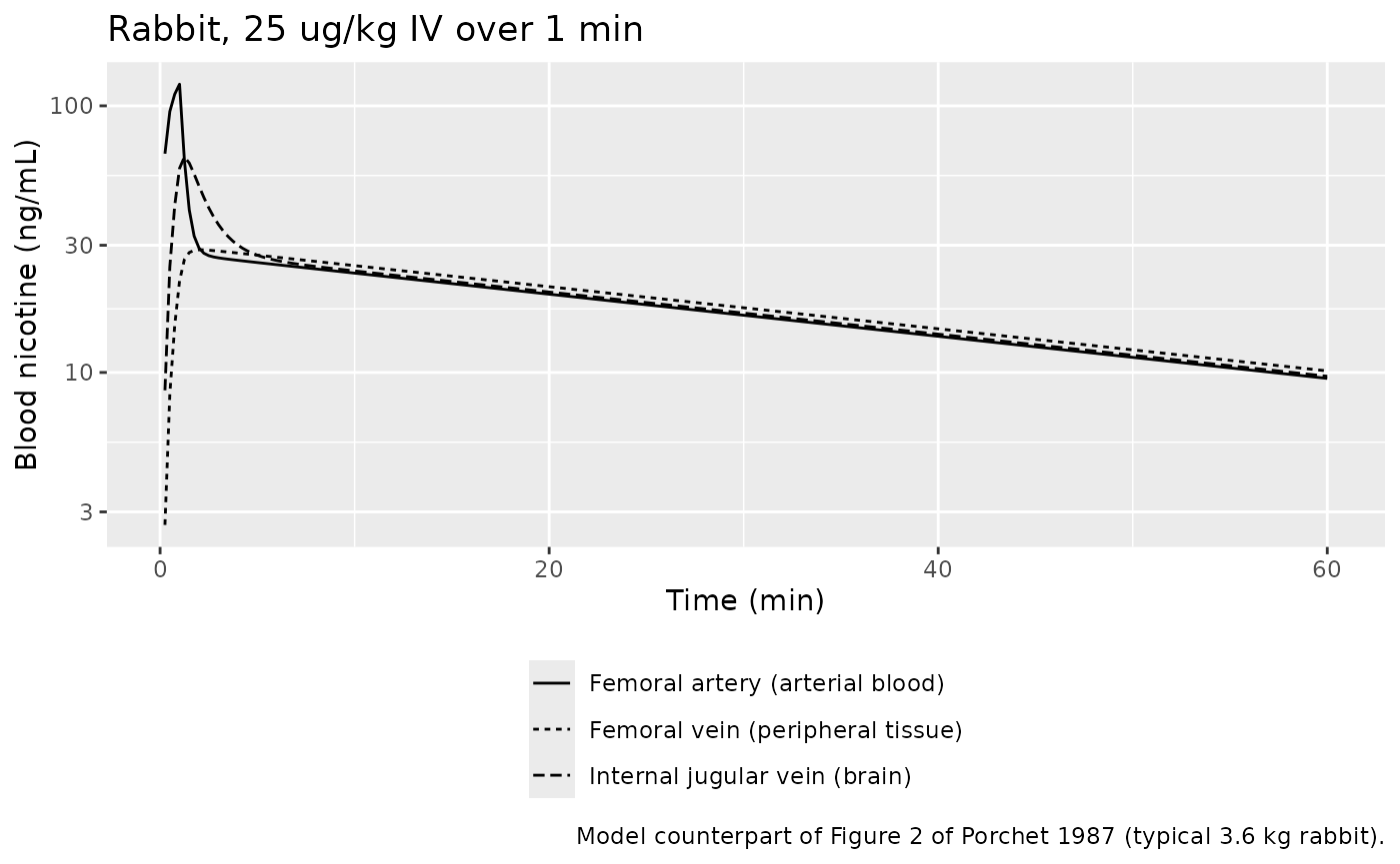
rab_at <- function(t) sim_rabbit[sim_rabbit$time == t, ]
stopifnot(
  # Femoral venous blood still rising while arterial and jugular fall early on
  # (Results): the femoral curve peaks after the end of the 1-min infusion.
  sim_rabbit$time[which.max(sim_rabbit$Cother)] > 1,
  sim_rabbit$time[which.max(sim_rabbit$Cbrain)] < sim_rabbit$time[which.max(sim_rabbit$Cother)],
  # Late phase: all three sites converge near the observed ~10 ng/mL at 60 min
  # (Figure 2), which the fitted clearance and peripheral PC control.
  abs(rab_at(60)$Cother / 10 - 1) < 0.25,
  abs(rab_at(60)$Cbrain / 10 - 1) < 0.25
)
The model reproduces the qualitative pattern the paper reports: the brain (jugular) curve peaks early and falls while femoral venous blood is still rising, and all three sites converge at about 10 ng/mL by 60 min. The arterial peak at 1 min (about 120 ng/mL here) is well below the observed mean of roughly 350 ng/mL; the authors fitted the triexponential to the mean data and judged only the jugular fit “satisfactory” (Figure 2 inset), describing the model as “only a crude approximation to reality”.
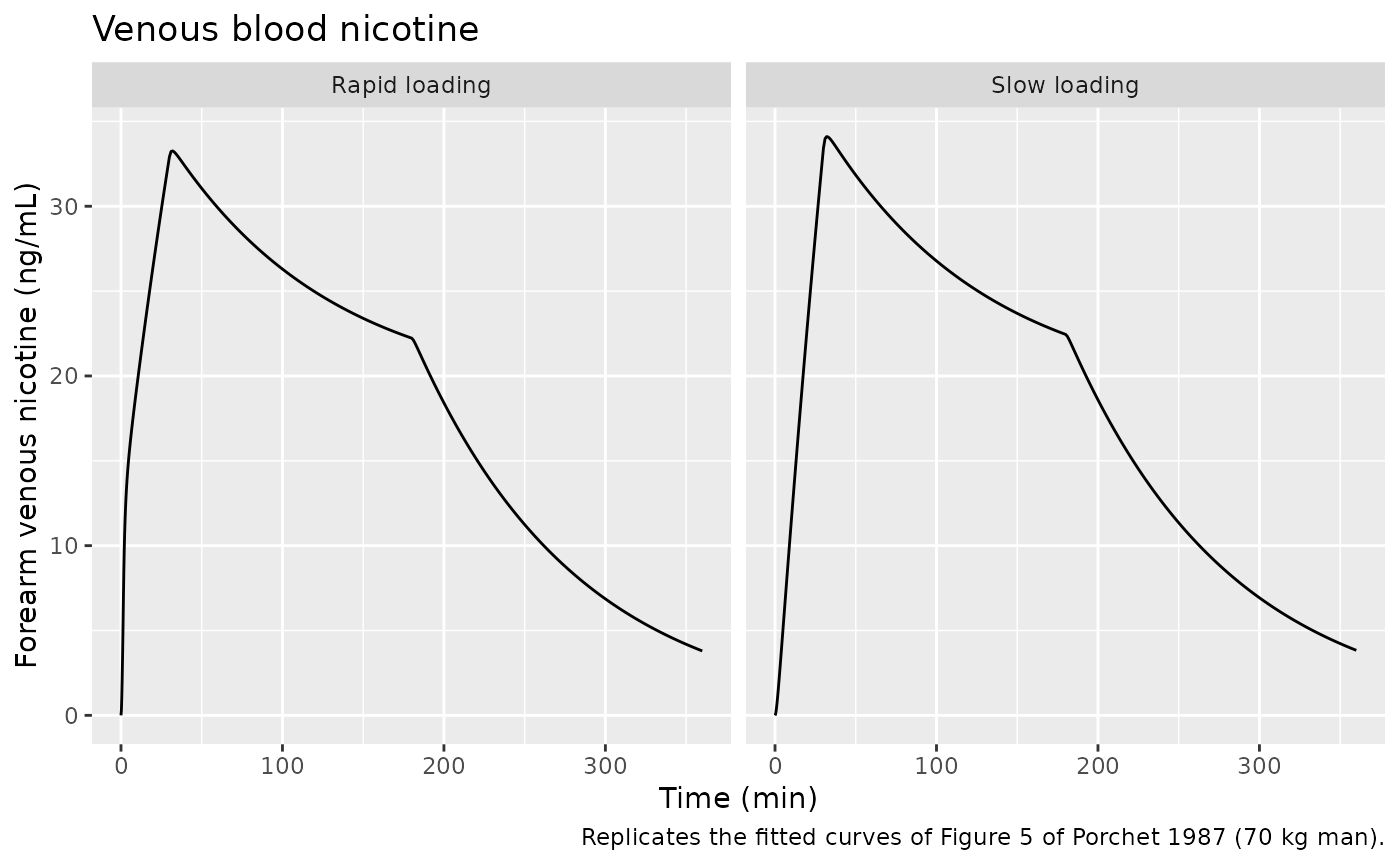
Human: venous and predicted brain concentrations (Figures 5 and 6)
mod_human <- readModelDb("Porchet_1987_nicotine_human_pbpk")
wt_human <- 70 # Table I physiology is that of a 70 kg man
obs_times <- sort(unique(c(seq(0, 10, by = 0.25), seq(10, 360, by = 1))))

# Each regimen: list of (rate in ug/kg/min, start, end).
regimens <- list(
  "Rapid loading" = list(c(17.5, 0, 1.5), c(1.75, 1.5, 30), c(0.35, 30, 180)),
  "Slow loading" = list(c(2.5, 0, 30), c(0.35, 30, 180))
)
make_regimen <- function(segments, id) {
  doses <- do.call(rbind, lapply(segments, function(s) {
    data.frame(time = s[2], amt = s[1] * wt_human * (s[3] - s[2]), dur = s[3] - s[2])
  }))
  dplyr::bind_rows(
    dplyr::mutate(doses, evid = 1L),
    data.frame(time = obs_times, amt = 0, dur = 0, evid = 0L)
  ) |>
    dplyr::mutate(id = id, cmt = "central") |>
    dplyr::arrange(time, dplyr::desc(evid))
}
ev_human <- dplyr::bind_rows(
  make_regimen(regimens[["Rapid loading"]], 1L) |> dplyr::mutate(regimen = "Rapid loading"),
  make_regimen(regimens[["Slow loading"]], 2L) |> dplyr::mutate(regimen = "Slow loading")
) |>
  dplyr::select(id, time, amt, dur, evid, cmt, regimen)
stopifnot(!anyDuplicated(unique(ev_human[, c("id", "time", "evid", "amt")])))

sim_human <- rxode2::rxSolve(mod_human, ev_human, keep = "regimen") |>
  as.data.frame()
sim_human |>
  ggplot(aes(time, Cother)) +
  geom_line() +
  facet_wrap(~regimen) +
  labs(
    x = "Time (min)", y = "Forearm venous nicotine (ng/mL)",
    title = "Venous blood nicotine",
    caption = "Replicates the fitted curves of Figure 5 of Porchet 1987 (70 kg man)."
  )
sim_human |>
  dplyr::filter(time <= 180) |>
  ggplot(aes(time, Cbrain, linetype = regimen)) +
  geom_line() +
  labs(
    x = "Time (min)", y = "'Brain' nicotine (ng/mL)", linetype = NULL,
    title = "Predicted brain nicotine",
    caption = "Replicates Figure 6 of Porchet 1987."
  ) +
  theme(legend.position = "bottom")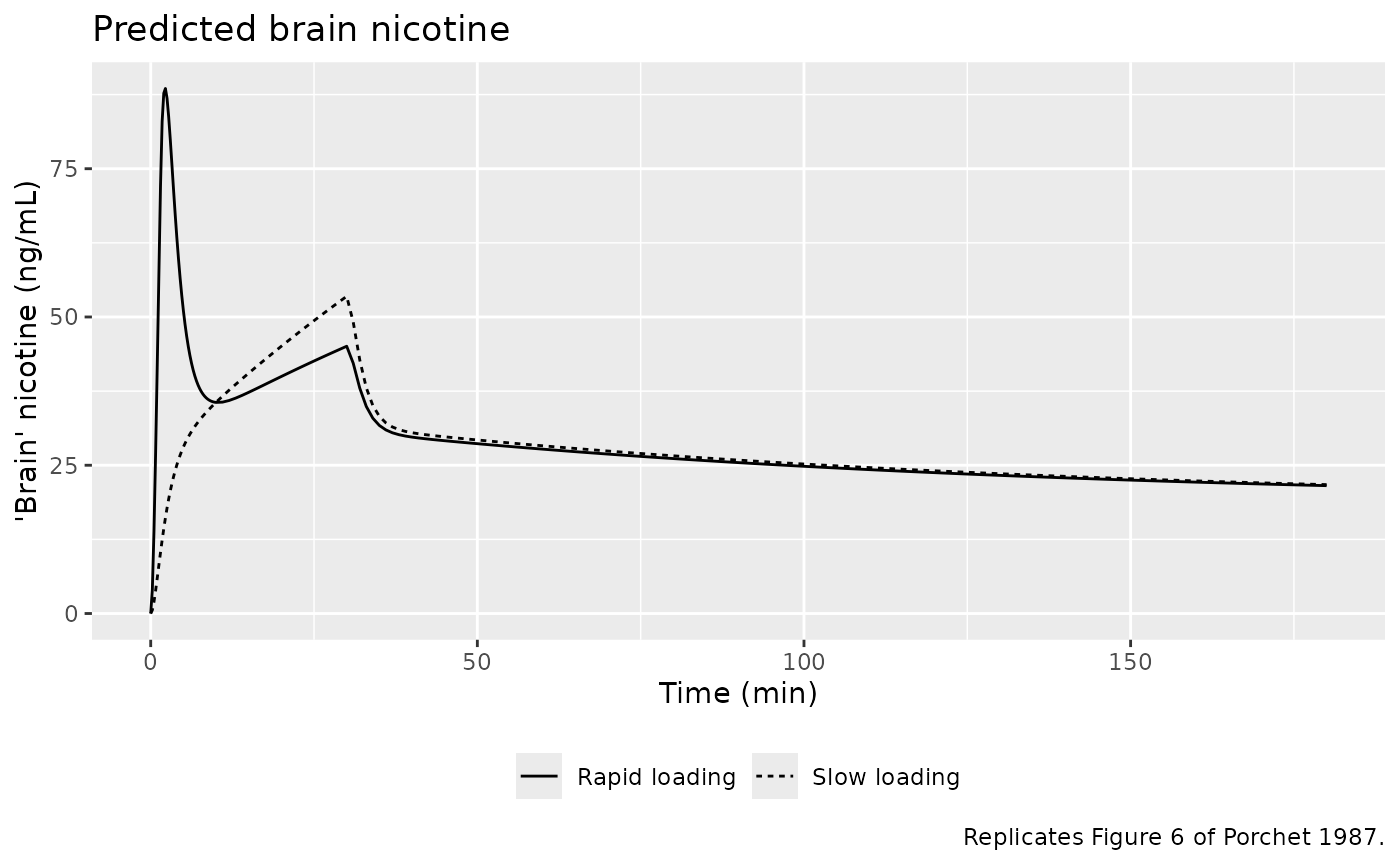
The predicted brain curve peaks within a few minutes of the start of rapid loading (about 88 ng/mL, matching the highest point of Figures 6 and 7 at roughly 80-85 ng/mL) and at the end of loading for the slow regimen, while venous blood peaks at the end of loading (30-32 min) for both regimens.
# Venous vs predicted brain concentration connected in time order: the
# clockwise venous loop that Figure 4 shows for heart rate is a distribution
# effect, which is why plotting effect against brain concentration (Figure 7)
# collapses it.
sim_human |>
  dplyr::filter(time <= 180) |>
  ggplot(aes(Cother, Cbrain, linetype = regimen)) +
  geom_path() +
  geom_abline(slope = 1, intercept = 0, colour = "grey60") +
  labs(
    x = "Forearm venous nicotine (ng/mL)", y = "'Brain' nicotine (ng/mL)",
    linetype = NULL,
    title = "Brain vs. venous nicotine, 0-180 min",
    caption = "Illustrates the distribution hysteresis behind Figures 4 and 7 of Porchet 1987."
  ) +
  theme(legend.position = "bottom")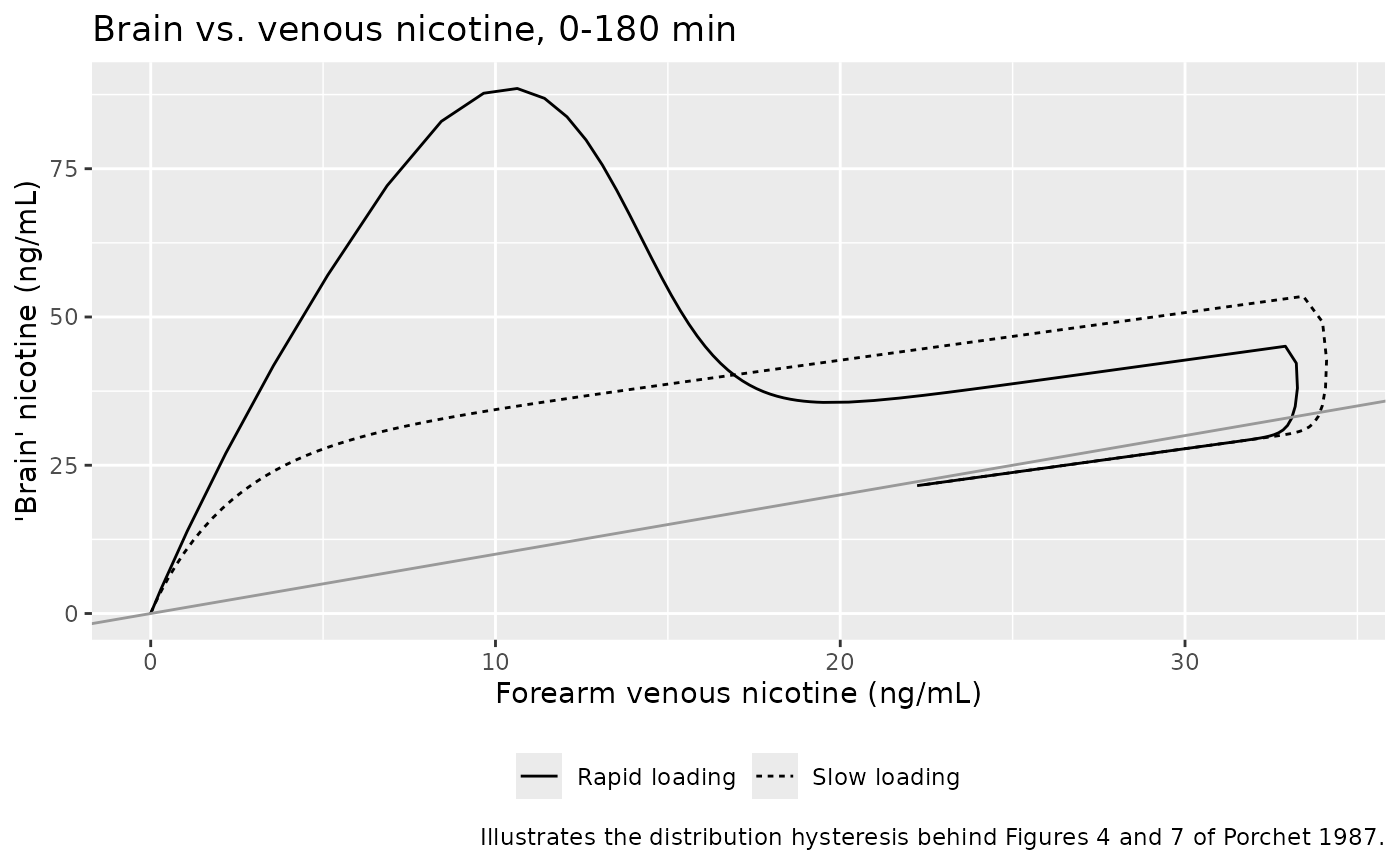
Peak times (Table III)
peak_times <- sim_human |>
  dplyr::group_by(regimen) |>
  dplyr::summarise(
    venous_tmax = time[which.max(Cother)],
    venous_cmax = max(Cother),
    brain_tmax = time[which.max(Cbrain)],
    brain_cmax = max(Cbrain),
    .groups = "drop"
  ) |>
  dplyr::mutate(
    venous_tmax_paper = c(30, 30),
    brain_tmax_paper = c(3, 30)
  )
peak_times |>
  dplyr::select(regimen, venous_tmax, venous_tmax_paper, brain_tmax, brain_tmax_paper) |>
  dplyr::rename(
    "Regimen" = regimen,
    "Venous Tmax, model (min)" = venous_tmax,
    "Venous Tmax, Table III (min)" = venous_tmax_paper,
    "Brain Tmax, model (min)" = brain_tmax,
    "Brain Tmax, Table III (min)" = brain_tmax_paper
  ) |>
knitr::kable(digits = 2, caption = "Time of peak venous and predicted brain nicotine.")| Regimen | Venous Tmax, model (min) | Venous Tmax, Table III (min) | Brain Tmax, model (min) | Brain Tmax, Table III (min) |
|---|---|---|---|---|
| Rapid loading | 32 | 30 | 2.25 | 3 |
| Slow loading | 32 | 30 | 30.00 | 30 |
stopifnot(
  # Venous blood peaks at the end of loading for both regimens (Table III:
  # 30 min, the sampling time). In the model peripheral blood lags the drop in
  # infusion rate and peaks at 32 min; a peak before 30 or after 33 min would
  # mean a wrong flow or partition coefficient.
  all(peak_times$venous_tmax >= 30 & peak_times$venous_tmax <= 33),
  # Brain peaks within the first 5 min of rapid loading (Table III: 3 min) and
  # at the end of slow loading (Table III: 30 min).
  peak_times$brain_tmax[peak_times$regimen == "Rapid loading"] <= 5,
  abs(peak_times$brain_tmax[peak_times$regimen == "Slow loading"] - 30) <= 1
)
The model’s rapid-loading brain peak falls at about 2 min; Table III reports 3 min, the nearest time at which the paper evaluated the prediction against heart rate. Venous blood peaks about 2 min after loading ends (32 min), because the peripheral tissue lags the drop to the maintenance rate; the paper’s 30 min is the sample nearest the peak.
PKNCA validation
The paper reports the observed maximum forearm venous concentration
(33.6 and 33.0 ng/mL for rapid and slow loading, at 30 min) and the
clearance computed as dose / AUC(0-inf) of venous blood (1,323 and 1,260
ml/min). The PKNCA block below computes the same quantities from the
simulated venous output. Because each regimen is several consecutive
infusions, the total dose is supplied to PKNCA as one dose record at
time zero; cl.obs is then total dose / AUC(0-inf).
sim_nca <- sim_human |>
  dplyr::filter(!is.na(Cother)) |>
  dplyr::select(id, time, Cother, regimen)
sim_nca <- dplyr::bind_rows(
  sim_nca,
  sim_nca |> dplyr::distinct(id, regimen) |> dplyr::mutate(time = 0, Cother = 0)
) |>
  dplyr::distinct(id, regimen, time, .keep_all = TRUE) |>
  dplyr::arrange(id, regimen, time)

conc_obj <- PKNCA::PKNCAconc(sim_nca, Cother ~ time | regimen + id)
dose_df <- ev_human |>
  dplyr::filter(evid == 1) |>
  dplyr::group_by(id, regimen) |>
  dplyr::summarise(amt = sum(amt), .groups = "drop") |>
  dplyr::mutate(time = 0)
dose_obj <- PKNCA::PKNCAdose(dose_df, amt ~ time | regimen + id)

intervals <- data.frame(
  start = 0, end = Inf,
  cmax = TRUE, tmax = TRUE, aucinf.obs = TRUE, cl.obs = TRUE, half.life = TRUE
)
nca_res <- PKNCA::pk.nca(PKNCA::PKNCAdata(conc_obj, dose_obj, intervals = intervals))

published <- tibble::tribble(
  ~regimen, ~cmax, ~tmax, ~cl.obs,
  "Rapid loading", 33.6, 30, 1.323,
  "Slow loading", 33.0, 30, 1.260
)
cmp <- nlmixr2lib::ncaComparisonTable(
  simulated = nca_res,
  reference = published,
  by = "regimen",
  units = c(cmax = "ng/mL", tmax = "min", cl.obs = "L/min"),
  tolerance_pct = 20
)
knitr::kable(cmp, caption = "Simulated vs. published venous NCA. * differs from reference by >20%.")| NCA parameter | regimen | Reference | Simulated | % diff |
|---|---|---|---|---|
| Cmax (ng/mL) | Rapid loading | 33.6 | 33.3 | -1.0% |
| Cmax (ng/mL) | Slow loading | 33 | 34.1 | +3.4% |
| Tmax (min) | Rapid loading | 30 | 32 | +6.7% |
| Tmax (min) | Slow loading | 30 | 32 | +6.7% |
| CL/F (L/min) | Rapid loading | 1.32 | 1.3 | -1.8% |
| CL/F (L/min) | Slow loading | 1.26 | 1.3 | +3.2% |
nca_wide <- as.data.frame(nca_res) |>
  dplyr::select(regimen, PPTESTCD, PPORRES) |>
  tidyr::pivot_wider(names_from = PPTESTCD, values_from = PPORRES) |>
  dplyr::left_join(published, by = "regimen", suffix = c("", "_paper"))
stopifnot(
  # Mass balance: venous AUC equals arterial AUC in this model, so dose/AUC
  # must return the encoded 1.3 L/min to within the trapezoid/extrapolation
  # error of the 0-360 min grid.
  all(abs(nca_wide$cl.obs / 1.3 - 1) < 0.03),
  # Observed venous Cmax (Results: 33.6 and 33.0 ng/mL).
  all(abs(nca_wide$cmax / nca_wide$cmax_paper - 1) < 0.10)
)
The simulated venous Cmax (33-34 ng/mL at 32 min for both regimens) and the dose / AUC clearance agree with the values reported in the Results. The clearance agreement is partly by construction: the human clearance was set to dose / venous AUC, and in this model the venous AUC equals the arterial AUC.
Assumptions and deviations
- No variability. Both models were fitted by extended least squares to mean concentration-time curves and the paper reports no between-subject or residual variance, so the models carry neither. They are typical-value models.
- Human body weight. The human doses are per kilogram and the subjects’ weights are not reported. The simulations use 70 kg, the body volume of the Table I human physiology (70,000 ml).
- Rabbit dose. The rabbit dose (25 ug/kg over 1 min) is simulated for the mean 3.6 kg rabbit as a 1-min infusion into arterial blood.
-
Rabbit
k21. Computingk21 = Q_periph / (V_periph x PC_periph)from Table I (760 ml/min, 3,587 ml) and Table II (PC_periph 0.729) gives 0.291/min, while Table II prints 0.298/min (andk31/k21= 3.312 instead of 3.40). The printed value would correspond to PC_periph of about 0.711. All human micro-constants and the other three rabbit micro-constants reproduce exactly, so the rabbit model is encoded with the paper’s primary parameters (Table II ’*’ rows) and Table I physiology. The 2.5 % gap is too small to change any conclusion. -
Human clearance. Table II marks the human clearance
(1,300 ml/min) as a primary parameter, but Methods state it was fixed to
dose / AUC(0-inf) of venous blood rather than fitted (Results: 1,323 and
1,260 ml/min for the two regimens). It is encoded as an estimable
lcl, notfixed(), because it was derived from the study data rather than from the literature. - Brain partition coefficient in man. Fixed to the rabbit estimate, as the paper assumes.
-
Observation sites. The paper identifies compartment
2 with femoral (rabbit) and forearm (human) venous blood and compartment
3 with internal jugular blood.
CotherandCbrainare therefore amount / apparent volume, the concentration in the blood leaving each tissue; the corresponding tissue concentration is that value times the partition coefficient. The predicted “brain” concentration in Figures 6 and 7 isCbrainon this definition: it reaches about 85 ng/mL after rapid loading in the paper and about 88 ng/mL in this model, whereas the tissue concentration would peak near 68 ng/mL. - Fitted human venous curve. Forearm venous blood was fitted with compartment 2: the published fitted curve (Figure 5) has no early spike, whereas arterial blood in this model reaches about 130 ng/mL in the first minute of rapid loading.
- No pharmacodynamic model. The paper reports that heart rate increases approximately linearly with predicted brain concentration (Figure 7) but fits no concentration-effect model and reports no slope, so no pharmacodynamic component is included.
- Errata. No correction notice for this article was found on PubMed as of 2026-10-11.