Gevokizumab mPBPK from aggregate data (Karakitsios 2024)
Source:vignettes/articles/Karakitsios_2024_gevokizumab.Rmd
Karakitsios_2024_gevokizumab.RmdModel and source
This paper contributes two models. Both share the Cao 2013 second-generation minimal PBPK (mPBPK) structure; they differ in which data were fitted and therefore in what the random effects mean.
- Single dosage group (7 mg IV, n = 10; Table 3): mPBPK. Second-generation minimal physiologically-based population PK model for gevokizumab (anti-interleukin-1beta humanized IgG2) in adults with type 2 diabetes, with between-subject variability estimated from AGGREGATE (mean and SD versus time) plasma concentration data rather than individual records. Karakitsios and Dokoumetzidis re-estimated the three drug-specific parameters of the Cao 2013 second-generation mPBPK structure (the tight- and leaky-tissue vascular reflection coefficients and plasma clearance) plus two IIV terms, using a Bayesian reconstruct-the-likelihood-from-aggregate-data method implemented in RStan: at each MCMC iteration a Latin-hypercube virtual population is solved, its mean and SD versus time are computed, and those summaries are fitted to the digitised published mean and SD profiles. This file holds the SINGLE dosage-group fit (7 mg IV, n = 10; Table 3). A single lognormal body-size random effect (etalvc) is shared by all four physiologic volumes, per the authors’ assumption that a larger patient has proportionally larger plasma, tight-tissue ISF, leaky-tissue ISF and lymph volumes. The five-dosage-group meta-analysis from the same paper is a separate model; see modellib(‘Karakitsios_2024_gevokizumab_mbma’).
- Five dosage groups, meta-analysis (Table 4): mPBPK / MBMA. Five-dosage-group meta-analysis of gevokizumab (anti-interleukin-1beta humanized IgG2) in adults with type 2 diabetes, fitted to AGGREGATE (mean and SD versus time) plasma concentration data from five dose arms simultaneously. The structural model is the Cao 2013 second-generation minimal PBPK model; Karakitsios and Dokoumetzidis estimated its three drug-specific parameters (tight- and leaky-tissue vascular reflection coefficients and plasma clearance) hierarchically, with an exponential INTER-GROUP variability (IGV) term on each, following a log-Student’s t distribution with 5 degrees of freedom to down-weight outlying dose arms. The random effects in this file are therefore DOSAGE-GROUP-level (eta_study_*), not between-subject: the model simulates group-mean concentration-time profiles and is NOT suitable for individual-subject simulation. Between-subject variability was estimated separately for each of the five arms (a semi-hierarchical design with no distribution assumed across arms), so no single population IIV exists; the five per-arm pairs are tabulated in population$notes. For an individual-level version of the same structure, see the single dosage-group fit modellib(‘Karakitsios_2024_gevokizumab’).
Citation: Karakitsios E, Dokoumetzidis A. A Meta-Analysis Methodology in Stan to Estimate Population Pharmacokinetic Parameters from Multiple Aggregate Concentration-Time Datasets: Application to Gevokizumab mPBPK Model. Pharmaceutics. 2024 Aug 27;16(9):1129. doi:10.3390/pharmaceutics16091129. Structural mPBPK equations and physiologic constants are those of Cao Y, Balthasar JP, Jusko WJ. J Pharmacokinet Pharmacodyn. 2013;40(5):597-607, reproduced in this paper’s Supplementary Material equations (S1)-(S8); see modellib(‘Cao_2013_gevokizumab’). Aggregate plasma data were digitised from Cavelti-Weder C et al. Diabetes Care. 2012;35(8):1654-1662 (PMID 22699287).
- Article: https://doi.org/10.3390/pharmaceutics16091129
- Supplement (equations S1-S8, Figure S1, traceplots S2-S8): https://www.mdpi.com/1999-4923/16/9/1129#supplementary
- Author source code: https://github.com/PMXathens/Gevokizumab
- Upstream structural model:
modellib("Cao_2013_gevokizumab")
What is unusual about this paper
The authors had no individual concentration records. They digitised the mean plasma concentration and its standard deviation versus time from a published graph (Cavelti-Weder 2012) and developed a Bayesian method that recovers population parameters from those aggregate summaries: at each MCMC iteration a Latin-hypercube virtual population is solved, its mean and SD versus time are computed, and those summaries are fitted to the digitised mean and SD profiles.
Two consequences shape this vignette:
- The residual error terms are aggregate-level.
sigma_1is the error between predicted and observed mean concentrations;sigma_2is the error on the SDs. Neither is an individual-level RUV, and the authors deliberately added no residual error to the virtual patients’ concentrations (Section 3.3). - Because the fitted quantity is a between-subject SD, the natural validation target is a predicted SD, not a predicted concentration. The paper prints one such observed/predicted pair, which is used below as an exact check.
Population
Fifty adults with type 2 diabetes from Cavelti-Weder 2012, in five single-dose intravenous arms of 10 patients each: 0.01, 0.03, 0.1, 0.3 and 1.0 mg/kg (0.7, 2.1, 7, 21 and 70 mg on a 70 kg basis). Plasma was sampled at 4, 8, 24, 48, 72, 96, 168, 216, 264, 336, 504, 672, 1008 and 1344 h after the dose (Section 2.1). A sixth published arm (3.0 mg/kg, n = 5) was excluded by the authors because 5 patients were considered too few to give accurate means and SDs (Section 2.4).
No individual demographics were recoverable from the digitised graph. All physiologic constants in the model are quoted for a 70 kg person, and the authors’ shared volume random effect is their proxy for unmeasured body-size differences.
The same information is available programmatically via
readModelDb("Karakitsios_2024_gevokizumab")()$population.
Source trace
Every ini() entry carries an in-file comment naming its
source location; the table collects them for review. “Supp.” refers to
the paper’s Supplementary Material.
| Equation / parameter | Value | Source location |
|---|---|---|
d/dt(plasma) |
n/a | Supp. equation (S1) (concentration form; encoded in amounts) |
d/dt(tight) |
n/a | Supp. equation (S2) |
d/dt(leaky) |
n/a | Supp. equation (S3) |
d/dt(lymph) |
n/a | Supp. equation (S4) |
vtight <- 0.65 * visf * kp |
n/a | Supp. equation (S7) |
vleaky <- 0.35 * visf * kp |
n/a | Supp. equation (S8) |
l1 <- 0.33 * lymphflow,
l2 <- 0.67 * lymphflow
|
n/a | Supp. text following equation (S4) |
sigmal (rcL) |
0.2 | Supp. text following equation (S4) |
kp |
0.8 | Supp. text following equation (S8) |
lymphflow (L) |
2.9 L/day = 2.9/24 L/h | Supp. text following equation (S8) |
visf (VISF) |
15.6 L | Supp. text following equation (S8) |
vlymph (Vlymph) |
5.2 L | Supp. text following equation (S8) |
lvc (Vplasma) |
2.6 L (fixed) | Supp. text following equation (S8) |
| Single dosage group (7 mg) | ||
sigma_tight (rc1_mean) |
0.9584 | Table 3 |
sigma_leaky (rc2_mean) |
0.7645 | Table 3 |
lcl (CLp_mean) |
0.0065 L/h | Table 3 |
etalcl (omega_CLp) |
0.0775 -> var 0.00600625 | Table 3 |
etalvc (omega_V) |
0.0699 -> var 0.00488601 | Table 3 |
expSd (sigma_1) |
0.0758 | Table 3 |
| (sigma_2, no individual analogue) | 0.2316 | Table 3 |
| Five dosage groups (meta-analysis) | ||
sigma_tight (rc1_mean) |
0.9504 | Table 4 |
sigma_leaky (rc2_mean) |
0.7674 | Table 4 |
lcl (CLp_mean) |
0.0064 L/h | Table 4 |
eta_study_lcl (gamma_CLp) |
0.1254 -> var 0.01572516 | Table 4 |
eta_study_sigma_tight (gamma_rc1) |
0.0338 -> var 0.00114244 | Table 4 |
eta_study_sigma_leaky (gamma_rc2) |
0.1810 -> var 0.032761 | Table 4 |
expSd (sigma_1) |
0.0734 | Table 4 |
| (sigma_2, no individual analogue) | 0.2706 | Table 4 |
Per-arm log_CLp, log_rc1,
log_rc2
|
see population$notes
|
Table 4 |
Per-arm omega_CLp, omega_V
|
see population$notes
|
Table 4 |
| IGV distribution (log-Student t, df = 5) | df fixed at 5 | Section 2.4 |
| IIV not applied to rc1 / rc2 | n/a | Section 2.2 |
| Digitised observed SDs, arm 4 | 0.31, 0.28, 0.57, 0.23, 0.18, 0.17 ug/mL | Section 3.2.2 |
| Paper’s predicted SD at the outlier point | 0.27 ug/mL | Section 3.2.2 / Figure 6b |
mod_one  <- readModelDb("Karakitsios_2024_gevokizumab")
mod_mbma <- readModelDb("Karakitsios_2024_gevokizumab_mbma")
Virtual cohort
The authors’ own inner loop is a Latin-hypercube sample over the two lognormal random effects, deliberately held fixed across MCMC iterations so that the predicted mean and SD are smooth functions of the parameters (Section 2.2). This vignette reproduces that idea with a deterministic midpoint-quantile factorial cohort: no seed, no Monte Carlo noise, and the predicted SD is reproducible to the last digit. Fourteen quantiles per random effect gives 196 subjects per arm, just under the 200-per-arm cap.
per_side <- 14L
zq <- stats::qnorm((seq_len(per_side) - 0.5) / per_side)

# Karakitsios 2024 Table 4: per-arm parameters (log scale) and per-arm IIV.
arms <- tibble::tribble(
  ~arm,          ~dose_mg, ~log_clp,  ~log_rc1, ~log_rc2, ~omega_clp, ~omega_v,
  "0.01 mg/kg",       0.7,  -5.0572,  -0.0588,  -0.4421,     0.1813,   0.1676,
  "0.03 mg/kg",       2.1,  -4.9818,  -0.0528,  -0.2947,     0.1138,   0.3213,
  "0.1 mg/kg",        7.0,  -5.0418,  -0.0441,  -0.2639,     0.0798,   0.0733,
  "0.3 mg/kg",       21.0,  -5.1067,  -0.0489,  -0.1878,     0.0374,   0.0960,
  "1.0 mg/kg",       70.0,  -5.1280,  -0.0513,  -0.2086,     0.2002,   0.1000
)

# Paper's sampling scheme (Section 2.1) plus a regular grid for the profiles.
obs_times <- sort(unique(c(
  0, 4, 8, 24, 48, 72, 96, 168, 216, 264, 336, 504, 672, 1008, 1344,
  seq(0, 1344, by = 24)
)))

make_arm <- function(arm_row, id_offset) {
  grid <- expand.grid(z_clp = zq, z_v = zq)
  subj <- tibble::tibble(
    id     = id_offset + seq_len(nrow(grid)),
    arm    = arm_row$arm,
    etalcl = arm_row$omega_clp * grid$z_clp,
    etalvc = arm_row$omega_v   * grid$z_v
  )
  dosing <- subj |>
    dplyr::mutate(time = 0, amt = arm_row$dose_mg, evid = 1L, cmt = "plasma")
  obs <- subj |>
    tidyr::crossing(time = obs_times) |>
    dplyr::mutate(amt = NA_real_, evid = 0L, cmt = "plasma")
  dplyr::bind_rows(dosing, obs) |>
    dplyr::arrange(id, time, dplyr::desc(evid))
}

events <- dplyr::bind_rows(lapply(seq_len(nrow(arms)), function(i) {
  make_arm(arms[i, ], id_offset = (i - 1L) * nrow(expand.grid(zq, zq)))
}))

stopifnot(!anyDuplicated(unique(events[, c("id", "time", "evid")])))
c(subjects_per_arm = nrow(expand.grid(zq, zq)), total_rows = nrow(events))
#> subjects_per_arm       total_rows
#>              196            58800
Simulation
Each arm has its own CLp, rc1 and
rc2, so each arm is solved with its own
params = override. omega = NA keeps rxode2
from drawing its own random effects, so the etalcl /
etalvc columns built above are the only source of
between-subject variability.
sim <- dplyr::bind_rows(lapply(seq_len(nrow(arms)), function(i) {
  a <- arms[i, ]
  ev <- events |> dplyr::filter(arm == a$arm)
  rxode2::rxSolve(
    mod_one, events = ev, omega = NA,
    params = c(lcl         = a$log_clp,
               sigma_tight = exp(a$log_rc1),
               sigma_leaky = exp(a$log_rc2)),
    keep = c("arm"), returnType = "data.frame"
  )
}))
#> ℹ parameter labels from comments will be replaced by 'label()'
#> Warning: multi-subject simulation without without 'omega'
#> Warning: multi-subject simulation without without 'omega'
#> Warning: multi-subject simulation without without 'omega'
#> Warning: multi-subject simulation without without 'omega'
#> Warning: multi-subject simulation without without 'omega'

sim$arm <- factor(sim$arm, levels = arms$arm)
aggregates <- sim |>
  dplyr::filter(!is.na(Cc), time > 0) |>
  dplyr::group_by(arm, time) |>
  dplyr::summarise(mean_cc = mean(Cc), sd_cc = stats::sd(Cc), .groups = "drop")
Replicate published results
Arm 4 predicted SDs versus the digitised observed SDs
This is the paper’s only printed observed-versus-predicted pair, and it is an exact end-to-end check of the whole encoding: the mPBPK equations, the L/day-to-L/h conversion, the per-arm parameters, and the shared volume random effect all have to be right for the number to land.
Section 3.2.2 reports that the digitised SDs for the fourth dosage group (0.3 mg/kg) were 0.31, 0.28, 0.57, 0.23, 0.18 and 0.17 ug/mL at 24, 48, 72, 96, 168 and 216 h, and that the 0.57 ug/mL point is an outlier because the model predicts 0.27 ug/mL there (Figure 6b).
arm4_obs <- tibble::tibble(
  time   = c(24, 48, 72, 96, 168, 216),
  obs_sd = c(0.31, 0.28, 0.57, 0.23, 0.18, 0.17)
)

arm4 <- aggregates |>
  dplyr::filter(arm == "0.3 mg/kg") |>
  dplyr::inner_join(arm4_obs, by = "time") |>
  dplyr::arrange(time) |>
  dplyr::mutate(pred_over_obs = sd_cc / obs_sd)

arm4 |>
  dplyr::select(time, mean_cc, sd_cc, obs_sd, pred_over_obs) |>
  dplyr::rename(
    "Time (h)"                      = time,
    "Predicted mean (ug/mL)"        = mean_cc,
    "Predicted SD (ug/mL)"          = sd_cc,
    "Digitised observed SD (ug/mL)" = obs_sd,
    "Predicted / observed"          = pred_over_obs
  ) |>
  knitr::kable(digits = 3,
               caption = paste("Arm 4 (0.3 mg/kg) predicted between-subject SDs versus the",
"digitised observed SDs reported in Section 3.2.2."))| Time (h) | Predicted mean (ug/mL) | Predicted SD (ug/mL) | Digitised observed SD (ug/mL) | Predicted / observed |
|---|---|---|---|---|
| 24 | 6.642 | 0.494 | 0.31 | 1.594 |
| 48 | 5.553 | 0.343 | 0.28 | 1.226 |
| 72 | 4.787 | 0.267 | 0.57 | 0.468 |
| 96 | 4.258 | 0.233 | 0.23 | 1.015 |
| 168 | 3.436 | 0.209 | 0.18 | 1.162 |
| 216 | 3.149 | 0.194 | 0.17 | 1.139 |
The predicted SD at 72 h reproduces the paper’s stated predicted value to the precision it was printed at. The authors’ argument for calling the 0.57 ug/mL observation an outlier is that the observed SD series should fall with time as the concentrations fall, and that this one point interrupts the decline. Both halves of that argument are checked below: the model’s predicted SDs decline monotonically, and 72 h is the only time at which the observed series rises.
The remaining time points sit within about 1.0 to 1.6 times the observed SDs. The largest of those, 1.59 at 24 h, is an over-prediction of the earliest and noisiest digitised point; it is reported here rather than treated as a target, since the arm’s variability terms come from the paper and were not adjusted.
pred_72 <- arm4$sd_cc[arm4$time == 72]
c(predicted_sd_72h = round(pred_72, 4), paper_value = 0.27)
#> predicted_sd_72h      paper_value
#>           0.2668           0.2700

# Gate: the paper prints 0.27 ug/mL to two decimals, so agreement to within
# half of the last printed digit is the tightest assertion the source supports.
stopifnot(abs(pred_72 - 0.27) < 0.005)

# Gate: the model's predicted SDs decline monotonically with time.
stopifnot(all(diff(arm4$sd_cc) < 0))

# Gate: the observed series rises at exactly one time point, 72 h -- which is
# the paper's stated reason for calling that value an outlier.
rises_at <- arm4$time[-1][diff(arm4$obs_sd) > 0]
stopifnot(length(rises_at) == 1L, rises_at == 72)
Mean and SD profiles for the five arms
Rendered in the style of the paper’s Figure 1 (predicted mean as a line, the predicted mean +/- SD band around it).
aggregates |>
  ggplot(aes(time, mean_cc)) +
  geom_ribbon(aes(ymin = pmax(mean_cc - sd_cc, 1e-4), ymax = mean_cc + sd_cc),
              alpha = 0.25, fill = "steelblue") +
  geom_line() +
  facet_wrap(~arm, scales = "free_y", nrow = 2) +
  scale_x_continuous(breaks = c(0, 336, 672, 1008, 1344)) +
  labs(x = "Time (h)", y = "Gevokizumab plasma concentration (mg/L = ug/mL)",
       caption = paste("Predicted mean (line) and mean +/- SD (band) per dosage group,",
                       "in the style of Figure 1 of Karakitsios 2024."))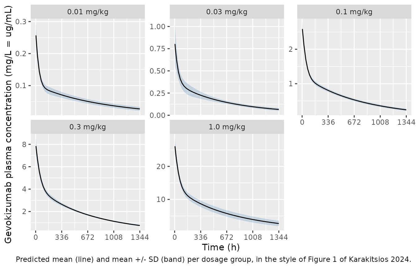
Re-estimated parameters versus Cao 2013
Section 3.2.2 compares the meta-analysis estimates with the values Cao et al. fitted to the same aggregate data by treating the mean profile as a single “mean patient”: CLp 0.0064 versus 0.00668 L/h, rc1 0.9504 versus 0.931, and rc2 0.7674 versus 0.837, the last being “moderately less” than Cao’s value.
comparison <- tibble::tribble(
  ~Parameter,        ~`Karakitsios 2024 (Table 4)`, ~`Cao 2013`,
  "CLp (L/h)",                             0.0064,      0.00668,
  "rc1 (tight tissues)",                   0.9504,      0.931,
  "rc2 (leaky tissues)",                   0.7674,      0.837
) |>
  dplyr::mutate(`Ratio` = `Karakitsios 2024 (Table 4)` / `Cao 2013`)

knitr::kable(comparison, digits = 4,
caption = "Meta-analysis estimates versus the Cao 2013 mean-patient fit.")| Parameter | Karakitsios 2024 (Table 4) | Cao 2013 | Ratio |
|---|---|---|---|
| CLp (L/h) | 0.0064 | 0.0067 | 0.9581 |
| rc1 (tight tissues) | 0.9504 | 0.9310 | 1.0208 |
| rc2 (leaky tissues) | 0.7674 | 0.8370 | 0.9168 |
Both parameterisations are packaged, so the effect on the predicted
profile can be seen directly. Cao_2013_gevokizumab uses
days as its time unit, so its profile is put on the same hour axis for
the comparison.
mod_cao <- readModelDb("Cao_2013_gevokizumab")

grid_h <- seq(0, 1344, by = 6)
ev_k <- rxode2::et(rxode2::et(amt = 7, cmt = "plasma"), grid_h)
ev_c <- rxode2::et(rxode2::et(amt = 7, cmt = "plasma"), grid_h / 24)

prof <- dplyr::bind_rows(
  rxode2::rxSolve(mod_mbma, ev_k, omega = NA, returnType = "data.frame") |>
    dplyr::transmute(time = time, Cc = Cc, model = "Karakitsios 2024 (five arms)"),
  # No `omega = NA` here: Cao_2013_gevokizumab is a typical-value model with
  # no etas at all, and rxSolve errors on omega = NA when there are none.
  rxode2::rxSolve(mod_cao, ev_c, returnType = "data.frame") |>
    dplyr::transmute(time = time * 24, Cc = Cc, model = "Cao 2013")
)
#> ℹ parameter labels from comments will be replaced by 'label()'

prof |>
  dplyr::filter(time > 0) |>
  ggplot(aes(time, Cc, colour = model)) +
  geom_line() +
  scale_y_log10() +
  labs(x = "Time (h)", y = "Gevokizumab plasma concentration (mg/L)",
       colour = NULL,
       caption = paste("Typical-value profiles after 7 mg IV under the two",
                       "parameterisations of the same mPBPK structure."))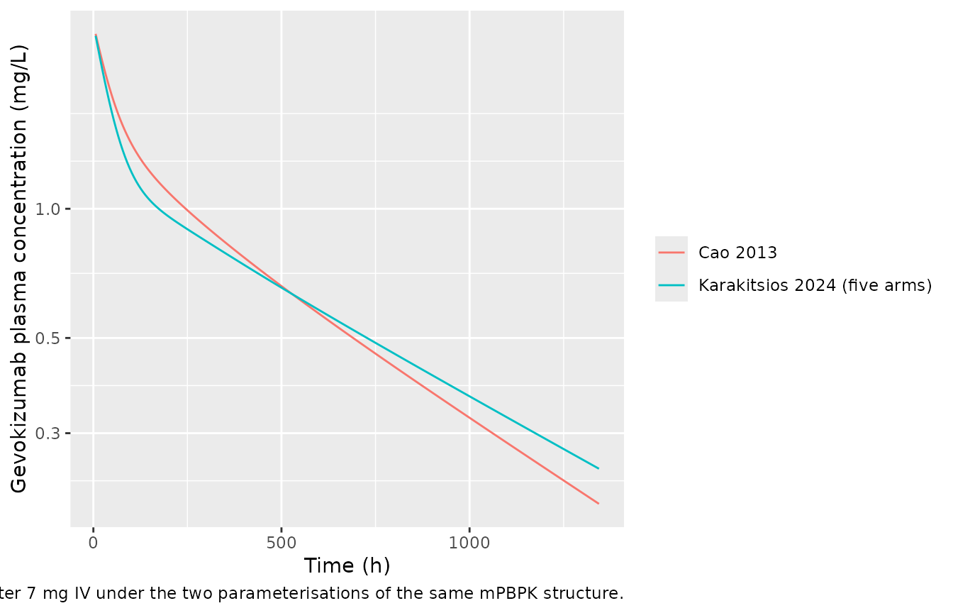
Inter-group variability in the meta-analysis model
The random effects of Karakitsios_2024_gevokizumab_mbma
are dosage-group-level, so a draw is a whole arm rather than a patient.
A deterministic 5 x 5 x 5 quintile factorial over the three IGV terms
gives 125 virtual dosage groups.
q5 <- stats::qnorm((seq_len(5) - 0.5) / 5)
igv <- expand.grid(z_cl = q5, z_rc1 = q5, z_rc2 = q5) |>
  dplyr::mutate(
    id                    = dplyr::row_number(),
    eta_study_lcl         = 0.1254 * z_cl,
    eta_study_sigma_tight = 0.0338 * z_rc1,
    eta_study_sigma_leaky = 0.1810 * z_rc2
  )

# The published exponential IGV on rc2 is unbounded above while the model's
# physiologic restriction (S6) requires rc2 < 1. Quantify the excursion.
rc2_draws <- 0.7674 * exp(igv$eta_study_sigma_leaky)
c(groups = nrow(igv),
  rc2_at_or_above_1 = sum(rc2_draws >= 1),
  normal_prob_rc2_above_1 =
    round(stats::pnorm(log(1 / 0.7674) / 0.1810, lower.tail = FALSE), 4))
#>                  groups       rc2_at_or_above_1 normal_prob_rc2_above_1
#>                125.0000                  0.0000                  0.0718

ev_igv <- dplyr::bind_rows(
  igv |> dplyr::transmute(id, time = 0, amt = 7, evid = 1L, cmt = "plasma",
                          eta_study_lcl, eta_study_sigma_tight, eta_study_sigma_leaky),
  igv |> tidyr::crossing(time = seq(0, 1344, by = 24)) |>
    dplyr::transmute(id, time, amt = NA_real_, evid = 0L, cmt = "plasma",
                     eta_study_lcl, eta_study_sigma_tight, eta_study_sigma_leaky)
) |>
  dplyr::arrange(id, time, dplyr::desc(evid))

sim_igv <- rxode2::rxSolve(mod_mbma, ev_igv, omega = NA, returnType = "data.frame")
#> Warning: multi-subject simulation without without 'omega'

sim_igv |>
  dplyr::filter(!is.na(Cc), time > 0) |>
  dplyr::group_by(time) |>
  dplyr::summarise(Q05 = stats::quantile(Cc, 0.05),
                   Q50 = stats::quantile(Cc, 0.50),
                   Q95 = stats::quantile(Cc, 0.95), .groups = "drop") |>
  ggplot(aes(time, Q50)) +
  geom_ribbon(aes(ymin = Q05, ymax = Q95), alpha = 0.25, fill = "darkorange") +
  geom_line() +
  scale_y_log10() +
  labs(x = "Time (h)", y = "Group-mean concentration (mg/L)",
       caption = paste("Between-dosage-group spread (5th-50th-95th percentile of 125",
                       "virtual arms) after 7 mg IV, from the Table 4 IGV terms."))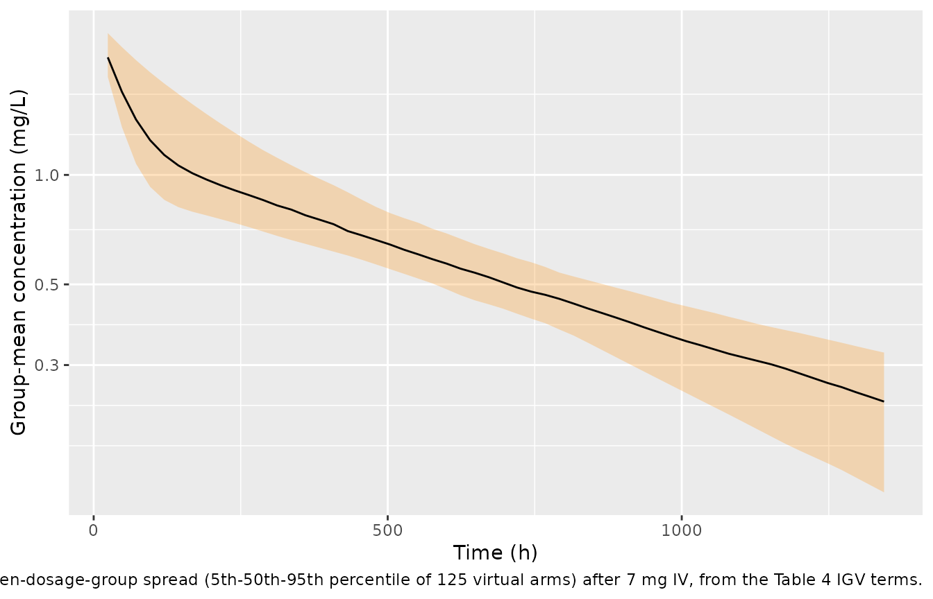
PKNCA validation
For a linear system two NCA quantities have exact closed forms, so they are ground truth rather than an approximate target:
-
AUC(0-inf) = Dose / CLpfor an intravenous dose, whatever the distribution structure. -
Vss = CLp * MRT, which for this mPBPK equalsVp + Vtight*(1-rc1)/(1-rcL) + Vleaky*(1-rc2)/(1-rcL) + Vlymph*(L1*(1-rc1) + L2*(1-rc2))/L, obtained by solving equations (S2)-(S4) at steady state.
Both identities cancel every parameter that NCA cannot see, so agreement confirms the ODE encoding and the unit conversion end to end. They are evaluated on typical-value profiles (one subject per arm) run out far enough for the terminal phase to be complete.
nca_grid <- sort(unique(c(seq(0, 2000, by = 1), seq(2000, 12000, by = 5))))

sim_typ <- dplyr::bind_rows(lapply(seq_len(nrow(arms)), function(i) {
  a <- arms[i, ]
  ev <- rxode2::et(rxode2::et(amt = a$dose_mg, cmt = "plasma"), nca_grid)
  rxode2::rxSolve(
    mod_one, ev, omega = NA,
    params = c(lcl         = a$log_clp,
               sigma_tight = exp(a$log_rc1),
               sigma_leaky = exp(a$log_rc2)),
    returnType = "data.frame", atol = 1e-10, rtol = 1e-10
  ) |>
    dplyr::transmute(id = i, arm = a$arm, time, Cc)
}))

sim_nca <- sim_typ |>
  dplyr::filter(!is.na(Cc)) |>
  dplyr::select(id, time, Cc, arm)

# A time-zero record must exist so PKNCA can anchor AUC. For an IV bolus the
# correct value at time zero is the post-dose concentration the solver already
# returns, NOT a synthetic zero, so this is asserted rather than back-filled.
stopifnot(all(tapply(sim_nca$time, sim_nca$id, min) == 0))

conc_obj <- PKNCA::PKNCAconc(sim_nca, Cc ~ time | arm + id)

dose_df <- arms |>
  dplyr::mutate(id = dplyr::row_number(), time = 0, amt = dose_mg, duration = 0) |>
  dplyr::select(id, time, amt, arm, duration)

dose_obj <- PKNCA::PKNCAdose(dose_df, amt ~ time | arm + id,
                             route = "intravascular", duration = "duration")

intervals <- data.frame(
  start = 0, end = Inf,
  cmax = TRUE, tmax = TRUE, aucinf.obs = TRUE,
  half.life = TRUE, mrt.iv.obs = TRUE, vss.iv.obs = TRUE, cl.obs = TRUE
)

nca_res <- PKNCA::pk.nca(PKNCA::PKNCAdata(conc_obj, dose_obj, intervals = intervals))
Comparison against the exact analytic identities
The paper reports no NCA table, so the reference column is the closed-form value implied by each arm’s own parameters – an exact target, not a digitised one.
rc_l <- 0.2; v_p <- 2.6; v_isf <- 15.6; k_p <- 0.8; v_lymph <- 5.2
v_tight <- 0.65 * v_isf * k_p
v_leaky <- 0.35 * v_isf * k_p

analytic <- arms |>
  dplyr::mutate(
    clp  = exp(log_clp),
    rc1  = exp(log_rc1),
    rc2  = exp(log_rc2),
    aucinf.obs = dose_mg / clp,
    vss.iv.obs = v_p +
      v_tight * (1 - rc1) / (1 - rc_l) +
      v_leaky * (1 - rc2) / (1 - rc_l) +
      v_lymph * (0.33 * (1 - rc1) + 0.67 * (1 - rc2)),
    cl.obs = clp
  ) |>
  dplyr::select(arm, aucinf.obs, vss.iv.obs, cl.obs)

cmp <- nlmixr2lib::ncaComparisonTable(
  simulated = nca_res,
  reference = analytic,
  by        = "arm",
  units     = c(aucinf.obs = "mg*h/L", vss.iv.obs = "L", cl.obs = "L/h"),
  tolerance_pct = 20
)

knitr::kable(cmp, digits = 4,
             caption = paste("Simulated NCA versus the exact closed-form values.",
"* marks a difference above 20%."))| NCA parameter | arm | Reference | Simulated | % diff |
|---|---|---|---|---|
| AUC0-∞ (obs) (mg*h/L) | 0.01 mg/kg | 110 | 110 | +0.0% |
| AUC0-∞ (obs) (mg*h/L) | 0.03 mg/kg | 306 | 306 | +0.0% |
| AUC0-∞ (obs) (mg*h/L) | 0.1 mg/kg | 1080 | 1080 | +0.0% |
| AUC0-∞ (obs) (mg*h/L) | 0.3 mg/kg | 3470 | 3470 | +0.0% |
| AUC0-∞ (obs) (mg*h/L) | 1.0 mg/kg | 11800 | 11800 | +0.0% |
| CL/F (L/h) | 0.01 mg/kg | 0.00636 | 0.00636 | -0.0% |
| CL/F (L/h) | 0.03 mg/kg | 0.00686 | 0.00686 | -0.0% |
| CL/F (L/h) | 0.1 mg/kg | 0.00646 | 0.00646 | -0.0% |
| CL/F (L/h) | 0.3 mg/kg | 0.00606 | 0.00606 | -0.0% |
| CL/F (L/h) | 1.0 mg/kg | 0.00593 | 0.00593 | -0.0% |
| Vss (IV) (L) | 0.01 mg/kg | 6.47 | 6.47 | -0.0% |
| Vss (IV) (L) | 0.03 mg/kg | 5.49 | 5.49 | -0.0% |
| Vss (IV) (L) | 0.1 mg/kg | 5.19 | 5.19 | -0.0% |
| Vss (IV) (L) | 0.3 mg/kg | 4.7 | 4.7 | -0.0% |
| Vss (IV) (L) | 1.0 mg/kg | 4.88 | 4.88 | -0.0% |
nca_wide <- as.data.frame(nca_res) |>
  dplyr::filter(start == 0, is.infinite(end)) |>
  dplyr::select(arm, PPTESTCD, PPORRES) |>
  tidyr::pivot_wider(names_from = PPTESTCD, values_from = PPORRES) |>
  dplyr::left_join(analytic, by = "arm", suffix = c("_nca", "_exact"))

# Both identities should hold to well within a percent; the residual is
# trapezoidal discretisation of the observation grid, not model error.
gates <- nca_wide |>
  dplyr::transmute(
    arm,
    auc_ratio = aucinf.obs_nca / aucinf.obs_exact,
    vss_ratio = vss.iv.obs_nca / vss.iv.obs_exact,
    cl_ratio  = cl.obs_nca / cl.obs_exact
  )
knitr::kable(gates, digits = 6,
caption = "NCA / closed-form ratios. Exact agreement is 1.")| arm | auc_ratio | vss_ratio | cl_ratio |
|---|---|---|---|
| 0.01 mg/kg | 1.000001 | 0.999997 | 0.999999 |
| 0.03 mg/kg | 1.000001 | 0.999998 | 0.999999 |
| 0.1 mg/kg | 1.000001 | 0.999998 | 0.999999 |
| 0.3 mg/kg | 1.000001 | 0.999998 | 0.999999 |
| 1.0 mg/kg | 1.000001 | 0.999998 | 0.999999 |
Dose linearity
The model is linear in dose, so scaled profiles must coincide exactly. With per-arm parameters differing between arms, the check is run within one parameter set.
ev_a <- rxode2::et(rxode2::et(amt = 7,  cmt = "plasma"), seq(0, 1344, by = 6))
ev_b <- rxode2::et(rxode2::et(amt = 70, cmt = "plasma"), seq(0, 1344, by = 6))
c_a <- rxode2::rxSolve(mod_one, ev_a, omega = NA, returnType = "data.frame")$Cc
c_b <- rxode2::rxSolve(mod_one, ev_b, omega = NA, returnType = "data.frame")$Cc
max_dev <- max(abs(10 * c_a - c_b), na.rm = TRUE)
c(max_abs_deviation = signif(max_dev, 3))
#> max_abs_deviation
#>          3.39e-07
stopifnot(max_dev < 1e-4)
Mass balance
With clearance driven to zero, the four states must retain the whole dose for all time. This exercises the transcapillary and lymphatic fluxes against each other and would catch a sign error or a mismatched reflection coefficient in any of equations (S1)-(S4).
ev_mb <- rxode2::et(rxode2::et(amt = 7, cmt = "plasma"), seq(0, 5000, by = 5))
mb <- rxode2::rxSolve(mod_one, ev_mb, omega = NA, params = c(lcl = log(1e-9)),
                      returnType = "data.frame", atol = 1e-10, rtol = 1e-10)
total <- mb$plasma + mb$tight + mb$leaky + mb$lymph
c(min_total = signif(min(total), 10), max_total = signif(max(total), 10), dose = 7)
#> min_total max_total      dose
#>  6.999993  7.000000  7.000000
stopifnot(max(abs(total - 7)) < 1e-3)
Assumptions and deviations
-
The two residual error terms are aggregate-level, not
individual-level.
sigma_1(0.0758 for the single arm; 0.0734 for the meta-analysis) is the exponential error between predicted and observed mean concentrations, and is mapped onto the model’sexpSdlognormal observation error because that is the closest available structure.sigma_2(0.2316 / 0.2706), the error on the observed SDs, has no individual-level analogue and is therefore recorded inpopulation$notesand in the source-trace table above rather than inini(). The authors added no residual error at all to the virtual patients’ concentrations (Section 3.3), so neither term should be read as a conventional RUV estimate. -
The IGV terms are drawn from a normal, not a Student
t. The paper assumed a log-Student t distribution with df fixed
at 5 for the three group-level parameters, to down-weight outlying arms
(Section 2.4). nlmixr2’s
ini()random effects are normal, soKarakitsios_2024_gevokizumab_mbmareproduces the reported IGV standard deviations but with normal rather than t-distributed tails. The point estimates are unaffected; only the tail behaviour of a simulated group differs. - The exponential IGV on rc2 is unbounded above. Physiologic restriction (S6) requires rc2 < 1, but an exponential random effect with gamma_rc2 = 0.1810 on a mean of 0.7674 exceeds 1 for about 7% of draws (see the IGV chunk, which counts them). Above 1 the transcapillary flux into leaky tissue changes sign, which is not physiologic. This is a property of the published parameterisation, so it is reproduced rather than clamped; users simulating from the IGV terms should filter such draws. The much smaller gamma_rc1 = 0.0338 on a mean of 0.9504 has the same issue for a smaller fraction of draws.
-
No population IIV exists for the meta-analysis
model. Between-subject variability was estimated separately for
each of the five arms, with no distribution assumed across arms (Section
2.4, “semi-hierarchical”). The five per-arm
omega_CLp/omega_Vpairs are tabulated inpopulation$notes; none of them is a population value, soini()inKarakitsios_2024_gevokizumab_mbmacarries only the group-level terms. Individual-level simulation should useKarakitsios_2024_gevokizumab, overridingetalcl/etalvcfor the arm of interest. -
Volumes carry a single shared random effect.
Section 2.2 states the same lognormal volume term is applied to all four
volumes, on the reasoning that a larger patient has proportionally more
plasma, tissue ISF and lymph. This is encoded as one
etalvcmultiplyingvplasma,visfandvlymph(and thereforevtightandvleaky, which are derived fromvisf), not as four independent random effects. -
No IIV on the reflection coefficients. The authors
tried this and found the resulting simulated SDs deviated substantially
from the observed ones (Section 2.2), so no eta is placed on
sigma_tightorsigma_leakyin either model. -
Time unit is hours, and lymph flow is converted.
The paper reports CLp in L/h and samples in hours, so
units$timeis"h"and theini()value is the published number unchanged. The physiologic lymph flow is published as 2.9 L/day, and appears inmodel()as2.9 / 24. The upstreamCao_2013_gevokizumabmodel uses days instead; both are internally consistent. -
Lymph volume differs from the packaged upstream
model. This paper’s Supplementary Material (text following
equation (S8)) states
Vlymph = 5.2 L, and that value is used here. The existingCao_2013_gevokizumabmodel file setsvlymph <- vplasma(2.6 L). Only the value stated by this paper’s own supplement was used; the discrepancy with the sibling file is flagged for separate review and was not changed here. - Cohort construction is deterministic, and smaller than the authors’. The authors predicted means and SDs from 1000 virtual patients, reduced to a 60-point Latin hypercube for speed. This vignette uses a 14 x 14 midpoint-quantile factorial (196 subjects per arm), which respects the 200-per-arm cap, needs no seed, and makes the predicted SD reproducible exactly. The arm 4 gate above shows this is accurate enough to land on the paper’s printed predicted SD.
-
No individual demographics were available. The
digitised aggregate data carry no weights, ages, sexes or races, so
covariateDatais empty for both models and body weight is recorded incovariatesDataExcludedas the implicit 70 kg basis of the physiologic constants rather than as a model covariate. - The 3.0 mg/kg arm is absent. The authors excluded the published sixth arm (n = 5) as too small for reliable means and SDs (Section 2.4), so it is not represented in either model or in this vignette.
- All parameter values come from the paper or its own supplement. No value was taken from a generic default or from another publication: the structural equations and physiologic constants are read from this paper’s Supplementary Material equations (S1)-(S8), and every estimate from Table 3 or Table 4.