Amoxicillin in healthy and critically ill dogs (Vegas Comitre 2021) • nlmixr2lib

Model and source

mod <- readModelDb("VegasComitre_2021_amoxicillin_dog")
ui <- rxode2::rxode(mod)
#> ℹ parameter labels from comments will be replaced by 'label()'
#> Warning: some etas defaulted to non-mu referenced, possible parsing error: etaiov_cl_1, etaiov_cl_2, etaiov_cl_3, etaiov_cl_4
#> as a work-around try putting the mu-referenced expression on a simple line

Citation: Vegas Comitre MD, Cortellini S, Cherlet M, Devreese M, Roques BB, Bousquet-Melou A, Toutain P-L, Pelligand L. (2021). Population Pharmacokinetics of Intravenous Amoxicillin Combined With Clavulanic Acid in Healthy and Critically Ill Dogs. Frontiers in Veterinary Science 8:770202. doi:10.3389/fvets.2021.770202.
Description: Veterinary (dog). Three-compartment population PK model for intravenous amoxicillin (given as amoxicillin-clavulanic acid) in 12 healthy laboratory beagles (single 20 mg/kg IV bolus) and 12 critically ill client-owned dogs in intensive care (20 mg/kg as a 0.5 h IV infusion every 8 h for at least 48 h), fitted jointly in Phoenix NLME. All disposition parameters are body-weight-normalised (L/kg, L/h/kg), so the dose supplied to this model is mg of amoxicillin per kg. Critical illness (DIS_CRITILL) lowers clearance to 43.6% of the healthy value and lowers the clearance to the superficial peripheral compartment by exp(-9.946), which removes that compartment from the disposition of sick dogs. Between-occasion variability on clearance applies to sick dogs only, with a larger variance on occasion 3. Residual error is combined additive plus proportional with separate magnitudes for healthy and sick dogs. Protein binding was negligible, so Cc is also the free concentration.
Article: https://doi.org/10.3389/fvets.2021.770202 (open access; PMC8636140)

The paper’s Supplementary Material (Data Sheet 1) holds only goodness-of-fit plots. The Results section says model code is included there too, but the published Data Sheet 1 has none. Every value in the model therefore comes from Table 4 and the Methods text.

Population

The two cohorts were modelled together in one Phoenix NLME fit (Tables 1 and 2).

Healthy dogs. Twelve intact female laboratory beagles from the Toulouse Veterinary School. Median age was 24 months and mean weight 11.5 kg (range 9.9-13.2). Each dog got a single IV bolus of amoxicillin-clavulanic acid (AMC) 20 mg/kg, which is 16.95 +/- 0.37 mg/kg of amoxicillin. Plasma was sampled at 0, 0.03, 0.17, 0.42, 0.67, 1, 2, 4, 6, 8, 10 and 12 h.
Critically ill dogs. Twelve client-owned, mixed-breed dogs in the intensive care unit of the Royal Veterinary College. Mean age was 40.2 months (range 4.8-114) and mean weight 20.6 kg (range 11.4-42.0). The cohort was 4 male, 6 male neutered, 1 female and 1 female spayed dog. Diagnoses were septic peritonitis (7), pyothorax (3), acute haemorrhagic diarrhoea syndrome (1) and burns (1). Two dogs had acute kidney injury and one was mechanically ventilated. Eleven of the 12 met SIRS criteria. The dogs got AMC 20 mg/kg (16.667 mg/kg amoxicillin) as a 0.5 h infusion every 8 h for at least 48 h. Sampling started after at least two doses. Samples were taken at the end of the infusion, then at 1, 2 and 4 h, with troughs at 8, 24 and 48 h.

In total, 218 amoxicillin concentrations were available (LLOQ 50 ng/mL, handled with the M3 method). Protein binding measured by ultrafiltration was negligible, so total concentration is also the free concentration.

The same information is available programmatically via readModelDb("VegasComitre_2021_amoxicillin_dog")()$population.

Source trace

Equation / parameter	Value	Source location
Three-compartment model, IV input into central	n/a	Results, ‘Population Pharmacokinetic Model’
`P_i = tvP * exp(eta_Pi)`	n/a	Methods Eq. (1)
`CV% = 100 * sqrt(exp(omega^2) - 1)`	n/a	Methods Eq. (2)
`lcl` (Cl, healthy)	0.336 L/h/kg	Table 4
`lvc` (V1)	0.173 L/kg	Table 4
`lq` (Cl2, superficial, healthy)	0.861 L/h/kg	Table 4
`lvp` (V2, superficial)	0.174 L/kg	Table 4
`lq2` (Cl3, deep)	0.0373 L/h/kg	Table 4
`lvp2` (V3, deep)	0.0776 L/kg	Table 4
`e_dis_critill_cl`	-0.829	Table 4, theta(Health) on Cl; footnote: sick Cl = healthy Cl x exp(-0.829)
`e_dis_critill_q`	-9.946	Table 4, theta(Health) on Cl2
`etalcl`	0.0399935 (20.2% CV)	Table 4, BSV Cl
`etalvc`	0.309251 (60.2% CV)	Table 4, BSV V1
`etalq`	0.164606 (42.3% CV)	Table 4, BSV Cl2
`etalvp`	0.00842838 (9.2% CV)	Table 4, BSV V2
`etaiov_cl_1`, `_2`, `_4`	0.0321307 (18.07% CV)	Table 4, BOV on Cl (all but Occasion 3)
`etaiov_cl_3`	0.16346 (42.14% CV)	Table 4, BOV on Cl (Occasion 3)
Occasion definitions	n/a	Methods, ‘Pharmacokinetic Analysis’ (estimation) and ‘Assessment of Dose-Exposure Relationship’ (simulation)
`propSd_healthy`	0.042	Table 4, proportional error healthy 4.2%
`addSd_healthy`	0.0306 mg/L	Table 4, additive error healthy 30.6 ng/mL
`propSd_critill`	0.359	Table 4, proportional error sick 35.9%
`addSd_critill`	0.00358 mg/L	Table 4, additive error sick 3.58 ng/mL
Combined additive + proportional residual error	n/a	Methods, ‘Pharmacokinetic Analysis’
Free fraction = 1	n/a	Results, ‘Protein Binding’

Typical-value check

The Table 4 footnote says that sick-dog clearance is 0.336 * exp(-0.829) = 0.147 L/h/kg, 43.6% of the control value. It also says that exp(-9.946) makes V2 unidentifiable in sick dogs. The model reproduces both.

tv <- with(as.list(ui$theta), c(
  cl_healthy = exp(lcl),
  cl_sick = exp(lcl + e_dis_critill_cl),
  q_healthy = exp(lq),
  q_sick = exp(lq + e_dis_critill_q)
))
signif(tv, 3)
#> cl_healthy    cl_sick  q_healthy     q_sick 
#>   3.36e-01   1.47e-01   8.61e-01   4.13e-05
stopifnot(
  abs(tv[["cl_sick"]] - 0.147) < 0.0005,
  abs(tv[["cl_sick"]] / tv[["cl_healthy"]] - 0.436) < 0.001,
  # Superficial compartment effectively disconnected: < 0.01% of healthy Cl2.
  tv[["q_sick"]] / tv[["q_healthy"]] < 1e-4
)

Virtual cohort and simulation

No individual data are published. Because the model is weight-normalised, each virtual dog needs only its health status (DIS_CRITILL) and, for sick dogs, the occasion index (OCC). Doses are mg of amoxicillin per kg. The paper’s Monte Carlo simulations used 1,000 dogs per population. Here, 200 per population and regimen are used.

# One cohort of n dogs on a regimen given as amoxicillin mg/kg per dose,
# infusion duration (h; 0 = bolus), dosing interval (h) and number of doses.
# Sick dogs use the paper's simulation occasions: 24-h blocks from the first
# dose (Methods, 'Assessment of Dose-Exposure Relationship').
make_cohort <- function(n, sick, amt, dur, ii, n_dose, obs_times,
                        id_offset = 0L, regimen = "") {
  ids <- id_offset + seq_len(n)
  dose_times <- (seq_len(n_dose) - 1) * ii
  doses <- expand.grid(id = ids, time = dose_times) |>
    mutate(evid = 1L, amt = amt, rate = if (dur > 0) amt / dur else 0)
  obs <- expand.grid(id = ids, time = obs_times) |>
    mutate(evid = 0L, amt = 0, rate = 0)
  bind_rows(doses, obs) |>
    mutate(
      cmt = "central",
      DIS_CRITILL = sick,
      OCC = pmin(floor(time / 24) + 1, 4),
      population = if (sick == 1) "Sick" else "Healthy",
      regimen = regimen
    ) |>
    arrange(id, time, desc(evid))
}

Figure 2: concentration-time profiles

The healthy dogs got one 16.95 mg/kg bolus. The sick dogs were dosed with 16.667 mg/kg as a 0.5 h infusion every 8 h. Their PK sampling interval was the third dose (16-24 h), matching Figure 1 (“the first plasma concentration was measured 16 to 24 h thereafter”). That interval is plotted against time after dose.

rxode2::rxSetSeed(20211115)
ev_vpc <- bind_rows(
  make_cohort(200, 0, amt = 16.95, dur = 0, ii = 24, n_dose = 1,
              obs_times = c(seq(0.02, 1, by = 0.02), seq(1.1, 12, by = 0.1)),
              id_offset = 0L),
  make_cohort(200, 1, amt = 16.667, dur = 0.5, ii = 8, n_dose = 7,
              obs_times = seq(16, 24, by = 0.1), id_offset = 200L)
)
stopifnot(!anyDuplicated(unique(ev_vpc[, c("id", "time", "evid")])))
sim_vpc <- rxode2::rxSolve(mod, events = ev_vpc, keep = "population",
                           returnType = "data.frame")
#> ℹ parameter labels from comments will be replaced by 'label()'
#> Warning: some etas defaulted to non-mu referenced, possible parsing error: etaiov_cl_1, etaiov_cl_2, etaiov_cl_3, etaiov_cl_4
#> as a work-around try putting the mu-referenced expression on a simple line
vpc <- sim_vpc |>
  mutate(tad = ifelse(population == "Sick", time - 16, time)) |>
  filter(tad > 0) |>
  group_by(population, tad) |>
  summarise(
    Q10 = quantile(Cc, 0.10), Q50 = median(Cc), Q90 = quantile(Cc, 0.90),
    .groups = "drop"
  )
ggplot(vpc, aes(tad, Q50 * 1000)) +
  geom_ribbon(aes(ymin = Q10 * 1000, ymax = Q90 * 1000), alpha = 0.25, fill = "steelblue") +
  geom_line() +
  facet_wrap(~population) +
  scale_y_log10(limits = c(50, NA)) +
  labs(x = "Time after administration (h)",
       y = "Amoxicillin plasma concentration (ng/mL)",
       title = "Simulated 10th / 50th / 90th percentiles",
       caption = "Replicates Figure 2 of Vegas Comitre 2021 (sick left, healthy right in the paper).")
#> Warning: Removed 26 rows containing missing values or values outside the scale range
#> (`geom_ribbon()`).
#> Warning: Removed 4 rows containing missing values or values outside the scale range
#> (`geom_line()`).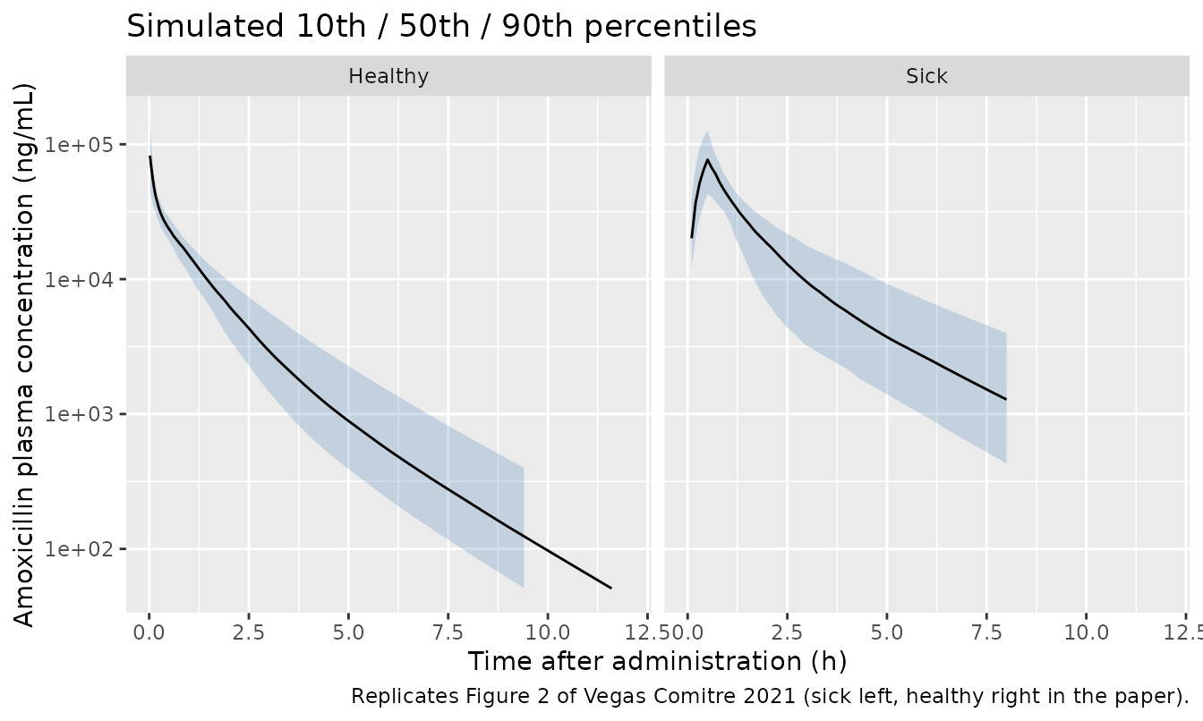

In Figure 2, observed concentrations are around 50,000 ng/mL shortly after dosing in both groups. At 8 h the observed median is about 2,000 ng/mL in sick dogs and a few hundred ng/mL in healthy dogs. The simulated bands follow the same shape. The sick-dog band is much wider than the healthy one, which reflects the larger proportional residual error and between-occasion variability of the ICU cohort.

Figure 3: time above MIC for seven regimens

For each regimen, the fraction of the 72-h treatment during which the free concentration exceeds the MIC (%fT > MIC) is computed on a 0.1 h grid. For each MIC, the plot shows the median and the value reached by 90% of dogs. The paper labels that value the “90th percentile” and it is the 10th percentile of %fT > MIC. The PK/PD cutoff (PK/PDCO) is the highest MIC at which 90% of dogs reach 40% fT > MIC.

regimens <- tribble(
  ~regimen,                        ~amt,   ~dur, ~ii,
  "A: 20 mg/kg q8h, 0.5 h",        16.667, 0.5,  8,
  "B: 20 mg/kg q8h, 1 h",          16.667, 1,    8,
  "C: 20 mg/kg q8h, 2 h",          16.667, 2,    8,
  "D: 20 mg/kg q8h, 3 h",          16.667, 3,    8,
  "E: 20 mg/kg q8h, 8 h CRI",      16.667, 8,    8,
  "F: 20 mg/kg q4h, 0.5 h",        16.667, 0.5,  4,
  "G: 40 mg/kg q8h, 0.5 h",        33.333, 0.5,  8
)
mics <- 2^(-4:5)
grid72 <- seq(0, 71.9, by = 0.1)

ft_one <- function(k) {
  r <- regimens[k, ]
  ev <- bind_rows(
    make_cohort(200, 0, r$amt, r$dur, r$ii, 72 / r$ii, grid72,
                id_offset = 0L, regimen = r$regimen),
    make_cohort(200, 1, r$amt, r$dur, r$ii, 72 / r$ii, grid72,
                id_offset = 200L, regimen = r$regimen)
  )
  s <- rxode2::rxSolve(mod, events = ev, keep = c("population", "regimen"),
                       returnType = "data.frame")
  s |>
    group_by(regimen, population, id) |>
    reframe(mic = mics, ft = vapply(mics, function(m) 100 * mean(Cc > m), numeric(1)))
}
rxode2::rxSetSeed(770202)
ft <- bind_rows(lapply(seq_len(nrow(regimens)), ft_one))

ft_sum <- ft |>
  group_by(regimen, population, mic) |>
  summarise(median = median(ft), p90 = quantile(ft, 0.10), .groups = "drop")

ft_sum |>
  pivot_longer(c(median, p90), names_to = "stat", values_to = "ft") |>
  mutate(curve = paste(population, ifelse(stat == "median", "median", "90th percentile"))) |>
  ggplot(aes(mic, ft, colour = curve)) +
  geom_line() +
  geom_hline(yintercept = 40, linetype = "dotted") +
  scale_x_continuous(trans = "log2", breaks = mics, labels = format(mics)) +
  scale_colour_manual(values = c(
    "Healthy median" = "forestgreen", "Healthy 90th percentile" = "darkorange",
    "Sick median" = "purple4", "Sick 90th percentile" = "orchid"
  )) +
  facet_wrap(~regimen, ncol = 2) +
  labs(x = "MIC (mg/L)", y = "free C > MIC (%) over 72 h", colour = NULL,
       caption = "Replicates Figure 3 of Vegas Comitre 2021 (panels A-G).") +
  theme(legend.position = "bottom", axis.text.x = element_text(angle = 90, size = 6))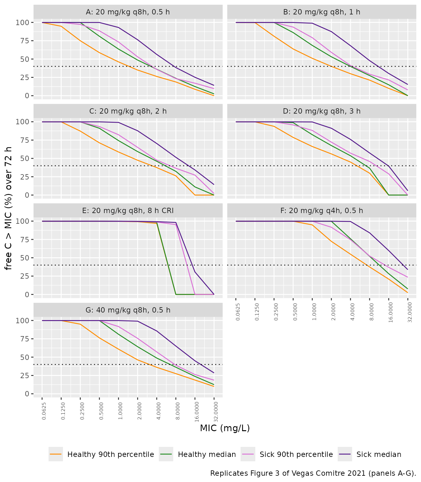

Comparison against Figure 3A

The standard-regimen curves below were read off Figure 3A by the maintainers. The readings are at the tabulated MICs and are good to about +/- 3 percentage points.

fig3a <- tribble(
  ~population, ~mic,  ~median_pub, ~p90_pub,
  "Healthy",   0.25,  100,         78,
  "Healthy",   0.5,   82,          62,
  "Healthy",   1,     65,          47,
  "Healthy",   2,     53,          36,
  "Healthy",   4,     40,          27,
  "Healthy",   8,     27,          17,
  "Healthy",   16,    13,          8,
  "Sick",      0.5,   100,         90,
  "Sick",      1,     96,          78,
  "Sick",      2,     83,          57,
  "Sick",      4,     63,          40,
  "Sick",      8,     43,          27,
  "Sick",      16,    28,          18,
  "Sick",      32,    15,          10
)
cmp3a <- ft_sum |>
  filter(regimen == regimens$regimen[1]) |>
  inner_join(fig3a, by = c("population", "mic")) |>
  mutate(d_median = median - median_pub, d_p90 = p90 - p90_pub)
cmp3a |>
  select(population, mic, median, median_pub, p90, p90_pub) |>
  mutate(mic = as.character(mic)) |>
  dplyr::rename(
    "Population" = population, "MIC (mg/L)" = mic,
    "Median, simulated" = median, "Median, Fig. 3A" = median_pub,
    "90th pct, simulated" = p90, "90th pct, Fig. 3A" = p90_pub
  ) |>
  knitr::kable(digits = 1, caption = "%fT > MIC over 72 h, standard regimen: simulated vs digitised Figure 3A.")

%fT > MIC over 72 h, standard regimen: simulated vs digitised Figure 3A.
Population	MIC (mg/L)	Median, simulated	Median, Fig. 3A	90th pct, simulated	90th pct, Fig. 3A
Healthy	0.25	99.9	100	75.0	78
Healthy	0.5	81.0	82	58.7	62
Healthy	1	63.6	65	46.1	47
Healthy	2	48.6	53	35.0	36
Healthy	4	36.1	40	26.2	27
Healthy	8	23.8	27	18.8	17
Healthy	16	12.5	13	8.8	8
Sick	0.5	99.9	100	88.5	90
Sick	1	93.1	96	73.3	78
Sick	2	76.3	83	53.0	57
Sick	4	56.3	63	35.8	40
Sick	8	38.4	43	23.3	27
Sick	16	25.1	28	17.0	18
Sick	32	14.1	15	9.7	10


# Centre and robust-envelope gates (per-dog tails differ across rxode2
# builds, so no single point is asserted). A mis-transcribed clearance or a
# unit error shifts every curve by tens of points.
all_d <- c(cmp3a$d_median, cmp3a$d_p90)
stopifnot(
  abs(median(all_d)) < 5,
  quantile(abs(all_d), 0.9) < 10
)

PK/PD cutoffs

pkpdco <- ft_sum |>
  group_by(regimen, population) |>
  summarise(PKPDCO = suppressWarnings(max(mic[p90 >= 40])), .groups = "drop") |>
  pivot_wider(names_from = population, values_from = PKPDCO)
published_co <- tribble(
  ~regimen,                     ~Healthy_pub, ~Sick_pub,
  "A: 20 mg/kg q8h, 0.5 h",     1,            4,
  "D: 20 mg/kg q8h, 3 h",       4,            8,
  "F: 20 mg/kg q4h, 0.5 h",     NA,           16
)
pkpdco |>
  left_join(published_co, by = "regimen") |>
  dplyr::rename(
    "Regimen" = regimen,
    "Healthy, simulated" = Healthy, "Healthy, paper" = Healthy_pub,
    "Sick, simulated" = Sick, "Sick, paper" = Sick_pub
  ) |>
  knitr::kable(caption = "PK/PDCO (mg/L; highest MIC with >= 40% fT > MIC in 90% of dogs). Paper values are those stated in the Results text.")

PK/PDCO (mg/L; highest MIC with >= 40% fT > MIC in 90% of dogs). Paper values are those stated in the Results text.
Regimen	Healthy, simulated	Sick, simulated	Healthy, paper	Sick, paper
A: 20 mg/kg q8h, 0.5 h	1	2	1	4
B: 20 mg/kg q8h, 1 h	2	4	NA	NA
C: 20 mg/kg q8h, 2 h	2	4	NA	NA
D: 20 mg/kg q8h, 3 h	4	8	4	8
E: 20 mg/kg q8h, 8 h CRI	4	8	NA	NA
F: 20 mg/kg q4h, 0.5 h	4	8	NA	16
G: 40 mg/kg q8h, 0.5 h	2	4	NA	NA

The paper states PK/PDCO values for regimens A, D and F in the text. For the other regimens, Figure 3 marks each crossing with an arrow but gives no number. The simulated cutoffs agree with the stated values to within one two-fold dilution. Regimen D matches exactly. The regimen A (sick) and regimen F cutoffs can come out one dilution lower. In each of those cases the paper’s 90th-percentile curve crosses 40% right at the stated cutoff MIC. The simulated curve reaches only about 35-39% there, while the simulated medians match the figure closely. A tail shortfall of a few percentage points therefore moves a statistic read on a two-fold grid by a whole dilution. The most likely cause is the unreported off-diagonal random-effect terms (see Assumptions and deviations). Cohort size may also contribute: 200 dogs per arm here, 1,000 in the paper.

PKNCA validation

The paper reports no NCA. Its derived clearances are 0.336 L/h/kg in healthy dogs and 0.147 L/h/kg in sick dogs (Abstract, Results). The volume at steady state follows from Table 4: V1 + V2 + V3 = 0.425 L/kg in healthy dogs. In sick dogs Cl2 is near zero, so V2 drops out and the volume is V1 + V3 = 0.251 L/kg. These are typical (median) values, so they can be checked against the median of a single-dose NCA. Sick dogs are simulated on one occasion (OCC = 1) so that clearance stays constant within each profile.

rxode2::rxSetSeed(8636140)
nca_times <- c(0, 0.03, 0.083, 0.17, 0.25, 0.42, 0.5, 0.67, 1, 1.5, 2, 3, 4,
               6, 8, 10, 12, 16, 24, 36, 48)
ev_nca <- bind_rows(
  make_cohort(200, 0, amt = 16.95, dur = 0, ii = 24, n_dose = 1,
              obs_times = nca_times, id_offset = 0L),
  make_cohort(200, 1, amt = 16.667, dur = 0.5, ii = 24, n_dose = 1,
              obs_times = nca_times, id_offset = 200L)
) |>
  mutate(OCC = 1, treatment = population)
# Post-dose concentrations below the assay LLOQ (50 ng/mL = 0.05 mg/L) are
# set to missing, as in the study. Without this, healthy-dog profiles fall to
# ~1e-7 mg/L by 36-48 h, and ODE round-off there (tiny negative values) breaks
# the lambda_z fit.
sim_nca <- rxode2::rxSolve(mod, events = ev_nca, keep = "treatment",
                           returnType = "data.frame") |>
  dplyr::mutate(Cc = ifelse(time > 0 & Cc < 0.05, NA_real_, Cc)) |>
  dplyr::filter(!is.na(Cc)) |>
  dplyr::select(id, time, Cc, treatment)
# Guarantee a time-zero row; for an IV dose the pre-dose concentration is 0.
sim_nca <- bind_rows(
  sim_nca,
  sim_nca |> distinct(id, treatment) |> mutate(time = 0, Cc = 0)
) |>
  distinct(id, treatment, time, .keep_all = TRUE) |>
  arrange(id, treatment, time)

dose_df <- ev_nca |>
  filter(evid == 1) |>
  mutate(duration = ifelse(rate > 0, amt / rate, 0)) |>
  select(id, time, amt, duration, treatment)

conc_obj <- PKNCA::PKNCAconc(sim_nca, Cc ~ time | treatment + id)
dose_obj <- PKNCA::PKNCAdose(dose_df, amt ~ time | treatment + id,
                             route = "intravascular", duration = "duration")
intervals <- data.frame(
  start = 0, end = Inf,
  cmax = TRUE, aucinf.obs = TRUE, half.life = TRUE,
  cl.obs = TRUE, vss.obs = TRUE
)
nca_res <- PKNCA::pk.nca(PKNCA::PKNCAdata(conc_obj, dose_obj, intervals = intervals))

published <- tribble(
  ~treatment, ~cl.obs, ~vss.obs,
  "Healthy",  0.336,   0.173 + 0.174 + 0.0776,
  "Sick",     0.147,   0.173 + 0.0776
)
cmp <- nlmixr2lib::ncaComparisonTable(
  simulated = nca_res,
  reference = published,
  by = "treatment",
  params = c("cl.obs", "vss.obs"),
  units = c(cl.obs = "L/h/kg", vss.obs = "L/kg"),
  tolerance_pct = 20
)
knitr::kable(cmp, caption = "Simulated single-dose NCA (median) vs the paper's typical clearance and Table 4 volumes. * differs by more than 20%.")

Simulated single-dose NCA (median) vs the paper’s typical clearance and Table 4 volumes. * differs by more than 20%.
NCA parameter	treatment	Reference	Simulated	% diff
CL/F (L/h/kg)	Healthy	0.336	0.331	-1.4%
CL/F (L/h/kg)	Sick	0.147	0.149	+1.4%
Vss/F (L/kg)	Healthy	0.425	0.432	+1.6%
Vss/F (L/kg)	Sick	0.251	0.275	+9.9%


nca_tab <- as.data.frame(nca_res$result) |>
  filter(PPTESTCD %in% c("cl.obs", "vss.obs")) |>
  group_by(treatment, PPTESTCD) |>
  summarise(med = median(PPORRES, na.rm = TRUE), n = sum(!is.na(PPORRES)), .groups = "drop")
med_of <- function(trt, p) nca_tab$med[nca_tab$treatment == trt & nca_tab$PPTESTCD == p]
stopifnot(
  # Nearly every profile must yield a clearance, or the median is meaningless.
  all(nca_tab$n >= 190),
  abs(med_of("Healthy", "cl.obs") / 0.336 - 1) < 0.10,
  abs(med_of("Sick", "cl.obs") / 0.147 - 1) < 0.10
)

The median NCA clearance matches the typical values. The volume comparison is looser because the 60% CV on V1 enters Vss additively, not multiplicatively. The median of the sum is therefore close to, but not exactly, the sum of the typical values.

Assumptions and deviations

Weight-normalised parameterisation. The paper estimates every volume and clearance per kg of body weight, and all doses are prescribed in mg/kg. The model keeps that form, so doses are mg of amoxicillin per kg. AMC 20 mg/kg corresponds to 16.667 mg/kg of amoxicillin. Concentrations are mg/L. The two additive residual SDs are converted from the paper’s ng/mL.
Diagonal random-effect matrix. The Methods say a full variance-covariance matrix was used for the Monte Carlo simulations, but Table 4 reports only the variances (as CV%). The off-diagonal terms are unknown and are set to zero. This is the most likely reason the simulated 90th-percentile (lower tail) %fT > MIC curves run a few percentage points below Figure 3 while the medians agree. Because of that, the PK/PDCO for regimen A (sick dogs) and regimen F (both populations) comes out one two-fold dilution below the published value.
Between-occasion variability. Table 4 describes BOV as that of sick dogs, and the paper’s simulations included it for sick dogs only, so the model gates it with DIS_CRITILL. Occasions 1, 2 and 4 share one variance (18.07% CV) and occasion 3 has its own (42.14% CV). In Table 4 the bootstrap medians of these two rows (47 and 19.4) look transposed relative to the estimates. The ‘Estimate’ column is used, which agrees with the Results text (“day-to-day variability much higher in Occasion 3”).
Occasion definition. For estimation the occasions were built around the 8-, 24- and 48-h troughs. The paper’s simulations, and this vignette, use 24-h blocks from the first dose. The model reads whatever occasion index is supplied in OCC. Any value outside 1-4 switches the BOV term off.
Residual error form. The Methods say only “a combination of additive and proportional error model”. The standard Phoenix additive-plus-multiplicative form, with variance add^2 + (prop * C)^2, is assumed. That is the same form as rxode2’s default add() + prop(). The paper estimated the error separately in healthy and sick dogs, and the model switches between the two sets with DIS_CRITILL.
Free concentration. Protein binding was negligible (Results, ‘Protein Binding’), so the %fT > MIC calculation uses Cc directly, as the paper did.
Confounding. Health status is fully confounded with breed, sex, weight and study site (healthy intact female beagles in Toulouse, sick mixed-breed dogs at the Royal Veterinary College). DIS_CRITILL carries all of these differences.
Figure 3 values in the comparison table were digitised by the maintainers from the published figure (about +/- 3 percentage points).
No correction notice for this article was found on the publisher’s page or in Crossref as of 2026-09-29.