Model and source
- Citation: Li X, Bo Y, Zeng Q, Diao L, Greene S, Patterson J, Liu L, Yang F (2024). Population pharmacokinetic model for oral ORIN1001 in Chinese patients with advanced solid tumors. Front Pharmacol 15:1322557. doi:10.3389/fphar.2024.1322557.
- Description: Two-compartment population PK model with first-order absorption and a lag time for oral ORIN1001 in Chinese patients with advanced solid tumors
- Article: https://doi.org/10.3389/fphar.2024.1322557
- Supplement (Data Sheet 1: Tables S1, Figures S1-S4, Equations S1-S3, full stepwise covariate log): https://www.frontiersin.org/articles/10.3389/fphar.2024.1322557/full#supplementary-material
ORIN1001 is a first-in-class oral inhibitor of the IRE1-alpha endoribonuclease, which blocks activation of the transcription factor XBP1 in the unfolded protein response. Li 2024 reports the first population PK model for the compound.
Population
Twenty-five Chinese adults with advanced solid tumors contributed 471 plasma ORIN1001 concentrations to the modeling dataset (Results 3.1). Subjects were enrolled in an open-label, dose-escalation and dose-expansion phase I basket trial (Register No. NCT05154201) approved by the Ethics Committee of Peking University Cancer Hospital. Seven dose groups received ORIN1001 tablets orally once daily at 100, 200, 300, 400, 500, 650, and 900 mg. Each subject was observed for 4 days following a single dose (single-dose period) and then through a 21-day once-daily cycle (multiple-dose period). Sampling was at 1, 2, 4, 6, 8, 12, 24, 48, 72, and 96 h in the single-dose period, and at 1, 2, 4, 6, 8, 12, and 24 h on day 21 in the multiple-dose period (Methods 2.1).
Baseline demographics and laboratory values are in Table 1: age 37-72 years (median 57), body weight 42-80 kg (median 64), 13 male / 12 female (48% female). The three covariates retained in the final model have cohort medians of lean body weight 45.13 kg (IQR 38.09-53.73, range 30-60.81), total bilirubin 10.30 umol/L (IQR 8.35-13.35, range 4.80-23.20), and lactate dehydrogenase 214 IU/L (IQR 180.50-279, range 98-1268). All subjects were Chinese.
The same information is available programmatically via the model’s
population metadata
(readModelDb("Li_2024_orin1001")()$population).
Source trace
The per-parameter origin is recorded as an in-file comment next to
each ini() entry in
inst/modeldb/specificDrugs/Li_2024_orin1001.R. The table
below collects them in one place for review. All values are the
final-model point estimates from Table 4; none were taken from the
bootstrap columns and none were taken from the base model (Supplementary
Table S1).
| Equation / parameter | Value | Source location |
|---|---|---|
lka |
0.58 1/h | Table 4, Ka, final-model estimate (17.12% RSE) |
ltlag |
0.35 h | Table 4, Tlag, final-model estimate (19.63% RSE) |
lvc |
26.21 L | Table 4, V/F, final-model estimate (5.39% RSE); Eq.
S2 |
lvp |
26.60 L | Table 4, V2/F, final-model estimate (9.72% RSE) |
lcl |
1.07 L/h | Table 4, CL/F, final-model estimate (5.31% RSE) |
lq |
0.75 L/h | Table 4, CL2/F, final-model estimate (12.57% RSE) |
e_tbili_cl |
-0.46 | Table 4, TBIL on CL/F; Eq. 3 |
e_lbm_cl |
1.11 | Table 4, LBW on CL/F; Eq. 3 |
e_lbm_q |
2.21 | Table 4, LBW on CL2/F; Eq. S1 |
e_ldh_vp |
0.99 | Table 4, LDH on V2/F; Eq. S3 |
etalka |
0.534 | Table 4, omega^2 Ka (a variance, per Table 4 footnote
a) |
etaltlag |
0.438 | Table 4, omega^2 Tlag
|
etalvc |
0.049 | Table 4, omega^2 V/F
|
etalcl |
0.067 | Table 4, omega^2 CL/F
|
propSd |
0.197 | Table 4, stdev0 (a standard deviation, per Table 4
footnote a); Results 3.2 states the intra-individual model was
proportional |
Exponential IIV, P = TVP * exp(eta)
|
n/a | Equation 1 |
| Median-normalized power covariate form | n/a | Equation 2 |
cl <- ... * (TBILI/10.3)^e_tbili_cl * (LBM/45.13)^e_lbm_cl |
n/a | Equation 3; medians from Table 1 |
q <- ... * (LBM/45.13)^e_lbm_q |
n/a | Equation S1 |
vc <- ... (no covariate) |
n/a | Equation S2 |
vp <- ... * (LDH/214)^e_ldh_vp |
n/a | Equation S3; median from Table 1 |
| Two-compartment, first-order absorption with lag, first-order elimination | n/a | Results 3.2 and Discussion paragraph 1 |
Retained covariate set CL/F-TBIL-LBW,
CL2/F-LBW, V2/F-LDH
|
n/a | Table 3 step 9 (final model); Supplementary stepwise log, scenario
cstep0323
|
The covariate reference values (10.3 umol/L, 45.13 kg, 214 IU/L) appear twice in the paper: as the Table 1 cohort medians and as the Figure 6 “Reference patients” definition. Both agree.
Virtual cohort
The original observed concentrations are not public. The cohort below is deterministic rather than randomly drawn: for each covariate, a lognormal distribution is fitted to the published median and interquartile range from Table 1, then evaluated at evenly spaced probability quantiles and clamped to the published min/max. This reproduces the published median and IQR exactly and makes the vignette’s numbers stable across runs. The three covariate vectors are rotated relative to one another so that they are not perfectly rank-correlated; the paper screened out covariate pairs with Pearson correlation above 0.5 (Methods 2.4.2), so weak correlation is the right target.
n_per <- 100L # participants per dose arm; the cohort cap is 200
doses <- c(100, 200, 300, 400, 500, 650, 900)

# Lognormal quantile matched to a published median + IQR, clamped to the
# published range.
qcov <- function(p, median, q1, q3, lo, hi) {
  sdlog <- log(q3 / q1) / (2 * stats::qnorm(0.75))
  pmin(pmax(median * exp(sdlog * stats::qnorm(p)), lo), hi)
}
# Deterministic rotation, used to decorrelate the covariate vectors without
# introducing a random draw.
rotate <- function(x, k) x[((seq_along(x) - 1L + k) %% length(x)) + 1L]

probs <- (seq_len(n_per) - 0.5) / n_per
LBM_vec <- qcov(probs, 45.13, 38.09, 53.73, 30, 60.81) # Table 1, LBW
TBILI_vec <- rotate(qcov(probs, 10.30, 8.35, 13.35, 4.80, 23.20), n_per %/% 3L)
LDH_vec <- rotate(qcov(probs, 214, 180.50, 279, 98, 1268), (2L * n_per) %/% 3L)

# The fitted cohort must reproduce the published medians.
stopifnot(
  abs(median(LBM_vec) - 45.13) < 0.05,
  abs(median(TBILI_vec) - 10.30) < 0.05,
  abs(median(LDH_vec) - 214) < 0.5,
  abs(cor(LBM_vec, TBILI_vec)) < 0.5,
  abs(cor(LBM_vec, LDH_vec)) < 0.5,
  abs(cor(TBILI_vec, LDH_vec)) < 0.5
)

subjects <- bind_rows(lapply(seq_along(doses), function(k) {
  tibble(
    id = (k - 1L) * n_per + seq_len(n_per),
    dose_mg = doses[k],
    cohort = paste0(doses[k], " mg"),
    LBM = LBM_vec,
    TBILI = TBILI_vec,
    LDH = LDH_vec
  )
}))
subjects$cohort <- factor(subjects$cohort, levels = paste0(doses, " mg"))

knitr::kable(
  tibble(
    Covariate = c("LBW (kg)", "TBIL (umol/L)", "LDH (IU/L)"),
    `Published median` = c(45.13, 10.30, 214),
    `Cohort median` = c(median(LBM_vec), median(TBILI_vec), median(LDH_vec)),
    `Published IQR` = c("38.09-53.73", "8.35-13.35", "180.50-279"),
    `Cohort IQR` = c(
      paste(round(quantile(LBM_vec, c(0.25, 0.75)), 2), collapse = "-"),
      paste(round(quantile(TBILI_vec, c(0.25, 0.75)), 2), collapse = "-"),
      paste(round(quantile(LDH_vec, c(0.25, 0.75)), 2), collapse = "-")
    )
  ),
  digits = 3,
  caption = "Virtual cohort covariates versus Li 2024 Table 1."
)| Covariate | Published median | Cohort median | Published IQR | Cohort IQR |
|---|---|---|---|---|
| LBW (kg) | 45.13 | 45.130 | 38.09-53.73 | 38.07-53.49 |
| TBIL (umol/L) | 10.30 | 10.300 | 8.35-13.35 | 8.17-12.99 |
| LDH (IU/L) | 214.00 | 214.002 | 180.50-279 | 172.56-265.39 |
Simulation
Observation rows use cmt = "central" (the ODE state);
Cc is returned as a column at those rows. Concentrations
from the model are in mg/L, i.e. ug/mL, because doses are in mg and
volumes in L. Li 2024 tabulates concentrations in ng/mL, so every
published value below has been divided by 1000 to put both scales in
ug/mL.
mod <- readModelDb("Li_2024_orin1001")

# Single-dose period: one 900 mg-class oral dose, sampled over 96 h per
# Methods 2.1.
obs_single <- c(0, 1, 2, 4, 6, 8, 12, 24, 48, 72, 96)
events_single <- bind_rows(
  subjects |> mutate(time = 0, amt = dose_mg, evid = 1L, cmt = "depot",
                     ii = 0, ss = 0L),
  subjects |> tidyr::crossing(time = obs_single) |>
    mutate(amt = NA_real_, evid = 0L, cmt = "central", ii = 0, ss = 0L)
) |>
  arrange(id, time, desc(evid))
stopifnot(!anyDuplicated(unique(events_single[, c("id", "time", "evid")])))

# Multiple-dose period: day 21 of once-daily dosing, sampled over one interval.
# The terminal half-life is long relative to the 24 h interval, so steady state
# is imposed with ss = 1 / ii = 24 rather than by dosing forward from zero.
obs_multi <- c(0, 1, 2, 4, 6, 8, 12, 24)
events_multi <- bind_rows(
  subjects |> mutate(time = 0, amt = dose_mg, evid = 1L, cmt = "depot",
                     ii = 24, ss = 1L),
  subjects |> tidyr::crossing(time = obs_multi) |>
    mutate(amt = NA_real_, evid = 0L, cmt = "central", ii = 0, ss = 0L)
) |>
  arrange(id, time, desc(evid))
stopifnot(!anyDuplicated(unique(events_multi[, c("id", "time", "evid")])))

set.seed(20240304)
sim_single <- rxode2::rxSolve(
  mod, events = as.data.frame(events_single),
  keep = c("cohort", "dose_mg", "LBM", "TBILI", "LDH")
) |>
  as.data.frame()
#> ℹ parameter labels from comments will be replaced by 'label()'

set.seed(20240304)
sim_multi <- rxode2::rxSolve(
  mod, events = as.data.frame(events_multi),
  keep = c("cohort", "dose_mg", "LBM", "TBILI", "LDH"),
  # steady-state searches for long-half-life subjects exceed the default step budget
  maxsteps = 1e6
) |>
  as.data.frame()
Cc is the individual prediction (IPRED). The
sim column additionally carries the proportional residual
error and is therefore the analogue of an observed concentration;
because Li 2024 ran its non-compartmental analysis on observed plasma
concentrations, the NCA sections below use sim.
Replicate published figures
# Replicates Figure 1 of Li 2024: observed ORIN1001 concentration-time
# profiles by dose group over the single-dose period.
sim_single |>
  filter(!is.na(Cc), time > 0) |>
  group_by(cohort, time) |>
  summarise(
    Q05 = quantile(sim, 0.05), Q50 = quantile(sim, 0.50),
    Q95 = quantile(sim, 0.95), .groups = "drop"
  ) |>
  ggplot(aes(time, Q50, colour = cohort, fill = cohort)) +
  geom_ribbon(aes(ymin = Q05, ymax = Q95), alpha = 0.15, colour = NA) +
  geom_line(linewidth = 0.7) +
  scale_y_log10() +
  labs(
    x = "Time after single dose (h)", y = "ORIN1001 (ug/mL)",
    colour = "Dose", fill = "Dose",
    title = "Single-dose concentration-time profiles by dose group",
    caption = "Replicates Figure 1 of Li 2024. Median with 5th-95th percentile band."
  )
#> Warning in scale_y_log10(): log-10 transformation introduced infinite values.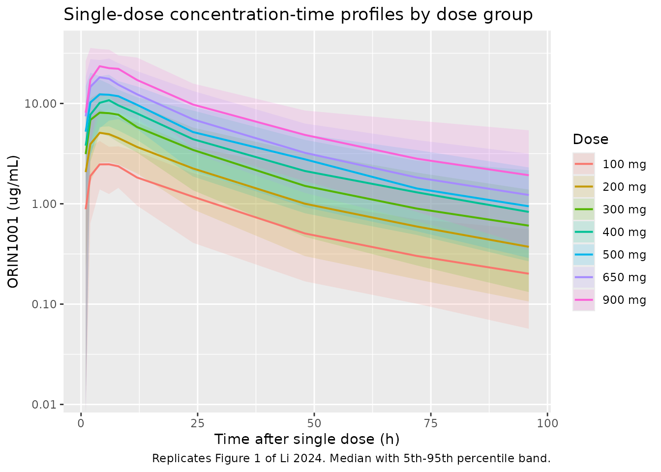
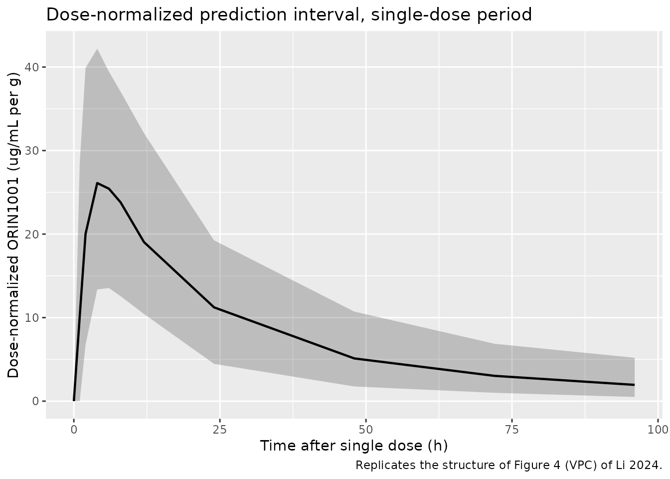
# Replicates Figure 4 of Li 2024: visual predictive check of the final model
# over the single-dose period, shown here as the simulated prediction interval.
sim_single |>
  filter(!is.na(Cc)) |>
  group_by(time) |>
  summarise(
    Q05 = quantile(sim / dose_mg * 1000, 0.05),
    Q50 = quantile(sim / dose_mg * 1000, 0.50),
    Q95 = quantile(sim / dose_mg * 1000, 0.95),
    .groups = "drop"
  ) |>
  ggplot(aes(time, Q50)) +
  geom_ribbon(aes(ymin = Q05, ymax = Q95), alpha = 0.25) +
  geom_line(linewidth = 0.8) +
  labs(
    x = "Time after single dose (h)",
    y = "Dose-normalized ORIN1001 (ug/mL per g)",
    title = "Dose-normalized prediction interval, single-dose period",
    caption = "Replicates the structure of Figure 4 (VPC) of Li 2024."
  )
PKNCA validation
Single-dose period
nca_single <- sim_single |>
  filter(!is.na(sim)) |>
  transmute(id, time, Cc = sim, cohort)

# Guarantee a time = 0 row per subject; pre-dose Cc = 0 is correct for an
# extravascular dose.
nca_single <- bind_rows(
  nca_single,
  nca_single |> distinct(id, cohort) |> mutate(time = 0, Cc = 0)
) |>
  distinct(id, cohort, time, .keep_all = TRUE) |>
  arrange(id, time)

conc_single <- PKNCA::PKNCAconc(
  nca_single, Cc ~ time | cohort + id, concu = "ug/mL", timeu = "h"
)
dose_single <- PKNCA::PKNCAdose(
  events_single |> filter(evid == 1L) |> select(id, time, amt, cohort) |>
    as.data.frame(),
  amt ~ time | cohort + id, doseu = "mg"
)

intervals_single <- data.frame(
  start = 0, end = Inf,
  cmax = TRUE, tmax = TRUE, auclast = TRUE, aucinf.obs = TRUE,
  half.life = TRUE, cl.obs = TRUE, vz.obs = TRUE
)
res_single <- suppressWarnings(PKNCA::pk.nca(
  PKNCA::PKNCAdata(conc_single, dose_single, intervals = intervals_single)
))

# PKNCA emits dependency rows for other intervals; filter on start/end as well
# as on the parameter so that only the requested 0-Inf interval is summarised.
sim_nca_single <- as.data.frame(res_single) |>
  filter(start == 0, is.infinite(end)) |>
  group_by(cohort, PPTESTCD) |>
  summarise(value = mean(PPORRES, na.rm = TRUE), .groups = "drop") |>
  tidyr::pivot_wider(names_from = PPTESTCD, values_from = value)
Li 2024 Table 2 reports arithmetic mean (SD) per dose group with n = 3-5, and Tmax as median (min, max). Concentrations and AUCs have been converted from ng/mL to ug/mL.
published_single <- tibble::tribble(
  ~cohort, ~cmax, ~tmax, ~auclast, ~aucinf.obs, ~half.life, ~cl.obs, ~vz.obs,
  "100 mg", 3.820, 2.00, 68.789, 75.963, 33.26, 1.34, 64.02,
  "200 mg", 5.590, 7.33, 131.729, 145.146, 32.01, 1.38, 63.74,
  "300 mg", 9.360, 4.00, 228.263, 255.483, 32.03, 1.20, 56.10,
  "400 mg", 13.447, 4.00, 368.183, 429.240, 33.68, 1.05, 48.56,
  "500 mg", 14.867, 4.33, 378.935, 423.553, 33.46, 1.18, 57.01,
  "650 mg", 18.300, 5.60, 522.604, 577.314, 29.74, 1.24, 51.51,
  "900 mg", 31.225, 11.50, 1043.135, 1188.790, 33.90, 0.90, 43.46
)

cmp_single <- nlmixr2lib::ncaComparisonTable(
  simulated = sim_nca_single |> mutate(cohort = as.character(cohort)),
  reference = published_single,
  by = "cohort",
  units = c(cmax = "ug/mL", auclast = "ug*h/mL", aucinf.obs = "ug*h/mL",
            tmax = "h", half.life = "h", cl.obs = "L/h", vz.obs = "L"),
  tolerance_pct = 20
)
knitr::kable(
  cmp_single,
  caption = paste(
    "Simulated versus published single-dose NCA (Li 2024 Table 2).",
    "* differs from the reference by >20%."
  )
)| NCA parameter | cohort | Reference | Simulated | % diff |
|---|---|---|---|---|
| Cmax (ug/mL) | 100 mg | 3.82 | 3.13 | -18.2% |
| Cmax (ug/mL) | 200 mg | 5.59 | 6.21 | +11.2% |
| Cmax (ug/mL) | 300 mg | 9.36 | 9.79 | +4.6% |
| Cmax (ug/mL) | 400 mg | 13.4 | 12.7 | -5.6% |
| Cmax (ug/mL) | 500 mg | 14.9 | 15.2 | +2.0% |
| Cmax (ug/mL) | 650 mg | 18.3 | 21.3 | +16.3% |
| Cmax (ug/mL) | 900 mg | 31.2 | 28.1 | -9.9% |
| Tmax (h) | 100 mg | 2 | 6.09 | +204.5%* |
| Tmax (h) | 200 mg | 7.33 | 5.93 | -19.1% |
| Tmax (h) | 300 mg | 4 | 5.32 | +33.0%* |
| Tmax (h) | 400 mg | 4 | 5.81 | +45.2%* |
| Tmax (h) | 500 mg | 4.33 | 5.55 | +28.2%* |
| Tmax (h) | 650 mg | 5.6 | 5.16 | -7.9% |
| Tmax (h) | 900 mg | 11.5 | 5.86 | -49.0%* |
| AUC0-∞ (obs) (ug*h/mL) | 100 mg | 76 | 93.3 | +22.9%* |
| AUC0-∞ (obs) (ug*h/mL) | 200 mg | 145 | 175 | +20.6%* |
| AUC0-∞ (obs) (ug*h/mL) | 300 mg | 255 | 277 | +8.4% |
| AUC0-∞ (obs) (ug*h/mL) | 400 mg | 429 | 375 | -12.6% |
| AUC0-∞ (obs) (ug*h/mL) | 500 mg | 424 | 446 | +5.2% |
| AUC0-∞ (obs) (ug*h/mL) | 650 mg | 577 | 592 | +2.5% |
| AUC0-∞ (obs) (ug*h/mL) | 900 mg | 1190 | 867 | -27.1%* |
| AUClast (ug*h/mL) | 100 mg | 68.8 | 80 | +16.3% |
| AUClast (ug*h/mL) | 200 mg | 132 | 155 | +17.8% |
| AUClast (ug*h/mL) | 300 mg | 228 | 245 | +7.3% |
| AUClast (ug*h/mL) | 400 mg | 368 | 327 | -11.1% |
| AUClast (ug*h/mL) | 500 mg | 379 | 391 | +3.3% |
| AUClast (ug*h/mL) | 650 mg | 523 | 521 | -0.2% |
| AUClast (ug*h/mL) | 900 mg | 1040 | 717 | -31.2%* |
| t½ (h) | 100 mg | 33.3 | 33.3 | +0.0% |
| t½ (h) | 200 mg | 32 | 29.5 | -7.9% |
| t½ (h) | 300 mg | 32 | 29.7 | -7.1% |
| t½ (h) | 400 mg | 33.7 | 31.4 | -6.7% |
| t½ (h) | 500 mg | 33.5 | 31.7 | -5.3% |
| t½ (h) | 650 mg | 29.7 | 29.2 | -2.0% |
| t½ (h) | 900 mg | 33.9 | 35.6 | +5.1% |
| CL/F (L/h) | 100 mg | 1.34 | 1.25 | -7.1% |
| CL/F (L/h) | 200 mg | 1.38 | 1.29 | -6.4% |
| CL/F (L/h) | 300 mg | 1.2 | 1.24 | +3.5% |
| CL/F (L/h) | 400 mg | 1.05 | 1.19 | +13.6% |
| CL/F (L/h) | 500 mg | 1.18 | 1.27 | +7.5% |
| CL/F (L/h) | 650 mg | 1.24 | 1.25 | +1.1% |
| CL/F (L/h) | 900 mg | 0.9 | 1.23 | +36.6%* |
| Vz/F (L) | 100 mg | 64 | 55.6 | -13.1% |
| Vz/F (L) | 200 mg | 63.7 | 53.1 | -16.7% |
| Vz/F (L) | 300 mg | 56.1 | 50.2 | -10.5% |
| Vz/F (L) | 400 mg | 48.6 | 50.8 | +4.6% |
| Vz/F (L) | 500 mg | 57 | 55.6 | -2.5% |
| Vz/F (L) | 650 mg | 51.5 | 49.3 | -4.3% |
| Vz/F (L) | 900 mg | 43.5 | 55.3 | +27.3%* |
Cmax and half-life reproduce across every dose group. The half-life agreement is the more informative of the two: the model’s true terminal half-life is longer than the value an NCA of this sampling design recovers.
# Analytic macro-constants at the reference covariate values.
kel <- 1.07 / 26.21
k12 <- 0.75 / 26.21
k21 <- 0.75 / 26.60
sum_k <- kel + k12 + k21
beta <- 0.5 * (sum_k - sqrt(sum_k^2 - 4 * kel * k21))
alpha <- 0.5 * (sum_k + sqrt(sum_k^2 - 4 * kel * k21))

tibble(
  Quantity = c(
    "Distribution half-life (analytic)",
    "Terminal half-life (analytic)",
    "Terminal half-life recovered by NCA over 0-96 h (simulated mean)",
    "Terminal half-life reported by Li 2024 (Table 2 range)"
  ),
  Value = c(
    sprintf("%.1f h", log(2) / alpha),
    sprintf("%.1f h", log(2) / beta),
    sprintf("%.1f h", mean(sim_nca_single$half.life)),
    "29.7-33.9 h"
  )
) |>
knitr::kable(caption = "Terminal half-life: model truth versus NCA estimate.")| Quantity | Value |
|---|---|
| Distribution half-life (analytic) | 8.3 h |
| Terminal half-life (analytic) | 50.5 h |
| Terminal half-life recovered by NCA over 0-96 h (simulated mean) | 31.5 h |
| Terminal half-life reported by Li 2024 (Table 2 range) | 29.7-33.9 h |
The model’s true terminal half-life is about 50 h, but a 96-hour sampling window places the log-linear regression on a segment that still contains distributional curvature, so the recovered value is roughly 30 h. The simulated NCA reproduces the paper’s reported 29.7-33.9 h precisely because it inherits the same estimator bias. Comparing the paper’s NCA half-life against the model’s analytic terminal half-life would have looked like a 50% error; comparing NCA to NCA shows there is none.
# Cmax and half-life must agree with Table 2 within the tolerance PKNCA
# comparison uses; these are the two columns least sensitive to the paper's
# small per-arm n.
chk <- sim_nca_single |>
  mutate(cohort = as.character(cohort)) |>
  inner_join(published_single, by = "cohort", suffix = c("_sim", "_pub"))
stopifnot(
  all(abs(chk$cmax_sim / chk$cmax_pub - 1) < 0.25),
  all(abs(chk$half.life_sim / chk$half.life_pub - 1) < 0.15)
)
Table 2 internal consistency
Before comparing the multiple-dose period, it is worth establishing
which estimator Li 2024 used. Every row of Table 2 – both periods –
satisfies Vz/F = (CL/F) / lambda_z with
lambda_z = log(2) / t_half. That identity holds only when
CL/F is computed as Dose / AUC(0-inf), so the
multiple-dose columns were produced by applying a single-dose-style
extrapolation to day-21 data rather than by a steady-state calculation.
This check also validates the transcription of the three interdependent
columns above.
table2 <- tibble::tribble(
  ~period, ~cohort, ~half.life, ~cl.obs, ~vz.obs,
  "Single", "100 mg", 33.26, 1.34, 64.02,
  "Single", "200 mg", 32.01, 1.38, 63.74,
  "Single", "300 mg", 32.03, 1.20, 56.10,
  "Single", "400 mg", 33.68, 1.05, 48.56,
  "Single", "500 mg", 33.46, 1.18, 57.01,
  "Single", "650 mg", 29.74, 1.24, 51.51,
  "Single", "900 mg", 33.90, 0.90, 43.46,
  "Multiple", "100 mg", 16.05, 0.99, 20.85,
  "Multiple", "200 mg", 20.19, 0.67, 18.65,
  "Multiple", "300 mg", 21.25, 0.68, 20.64,
  "Multiple", "400 mg", 25.53, 0.55, 18.76,
  "Multiple", "500 mg", 31.04, 0.40, 16.37,
  "Multiple", "650 mg", 18.91, 0.59, 16.29,
  "Multiple", "900 mg", 17.81, 0.57, 14.73
) |>
  mutate(vz_implied = cl.obs / (log(2) / half.life), ratio = vz_implied / vz.obs)

table2 |>
  select(period, cohort, half.life, cl.obs, vz.obs, vz_implied, ratio) |>
  dplyr::rename(
    "Period" = period, "Dose" = cohort, "t1/2 (h)" = half.life,
    "CL/F (L/h)" = cl.obs, "Vz/F (L), reported" = vz.obs,
    "Vz/F (L), (CL/F)/lambda_z" = vz_implied, "Ratio" = ratio
  ) |>
knitr::kable(digits = 3, caption = "Li 2024 Table 2 internal consistency.")| Period | Dose | t1/2 (h) | CL/F (L/h) | Vz/F (L), reported | Vz/F (L), (CL/F)/lambda_z | Ratio |
|---|---|---|---|---|---|---|
| Single | 100 mg | 33.26 | 1.34 | 64.02 | 64.299 | 1.004 |
| Single | 200 mg | 32.01 | 1.38 | 63.74 | 63.729 | 1.000 |
| Single | 300 mg | 32.03 | 1.20 | 56.10 | 55.451 | 0.988 |
| Single | 400 mg | 33.68 | 1.05 | 48.56 | 51.019 | 1.051 |
| Single | 500 mg | 33.46 | 1.18 | 57.01 | 56.962 | 0.999 |
| Single | 650 mg | 29.74 | 1.24 | 51.51 | 53.203 | 1.033 |
| Single | 900 mg | 33.90 | 0.90 | 43.46 | 44.017 | 1.013 |
| Multiple | 100 mg | 16.05 | 0.99 | 20.85 | 22.924 | 1.099 |
| Multiple | 200 mg | 20.19 | 0.67 | 18.65 | 19.516 | 1.046 |
| Multiple | 300 mg | 21.25 | 0.68 | 20.64 | 20.847 | 1.010 |
| Multiple | 400 mg | 25.53 | 0.55 | 18.76 | 20.258 | 1.080 |
| Multiple | 500 mg | 31.04 | 0.40 | 16.37 | 17.913 | 1.094 |
| Multiple | 650 mg | 18.91 | 0.59 | 16.29 | 16.096 | 0.988 |
| Multiple | 900 mg | 17.81 | 0.57 | 14.73 | 14.646 | 0.994 |
Multiple-dose period (day 21)
Because Table 2’s multiple-dose columns come from a single-dose-style
analysis of day-21 data, the same estimator is applied to the simulated
steady-state profile: the interval runs to Inf, so PKNCA
extrapolates beyond the last sample exactly as the paper’s software
did.
nca_multi <- sim_multi |>
  filter(!is.na(sim)) |>
  transmute(id, time, Cc = sim, cohort)

conc_multi <- PKNCA::PKNCAconc(
  nca_multi, Cc ~ time | cohort + id, concu = "ug/mL", timeu = "h"
)
dose_multi <- PKNCA::PKNCAdose(
  events_multi |> filter(evid == 1L) |> select(id, time, amt, cohort) |>
    as.data.frame(),
  amt ~ time | cohort + id, doseu = "mg"
)
intervals_multi <- data.frame(
  start = 0, end = Inf,
  cmax = TRUE, tmax = TRUE, cmin = TRUE, auclast = TRUE,
  half.life = TRUE, cl.obs = TRUE, vz.obs = TRUE
)
res_multi <- suppressWarnings(PKNCA::pk.nca(
  PKNCA::PKNCAdata(conc_multi, dose_multi, intervals = intervals_multi)
))
sim_nca_multi <- as.data.frame(res_multi) |>
  filter(start == 0, is.infinite(end)) |>
  group_by(cohort, PPTESTCD) |>
  summarise(value = mean(PPORRES, na.rm = TRUE), .groups = "drop") |>
  tidyr::pivot_wider(names_from = PPTESTCD, values_from = value)
published_multi <- tibble::tribble(
  ~cohort, ~cmax, ~tmax, ~auclast, ~vz.obs,
  "100 mg", 4.847, 3.33, 66.065, 20.85,
  "200 mg", 10.633, 4.67, 171.947, 18.65,
  "300 mg", 14.700, 4.00, 239.482, 20.64,
  "400 mg", 21.467, 4.00, 371.282, 18.76,
  "500 mg", 33.533, 4.33, 579.450, 16.37,
  "650 mg", 39.400, 2.00, 661.975, 16.29,
  "900 mg", 58.650, 5.00, 1022.700, 14.73
)

cmp_multi <- nlmixr2lib::ncaComparisonTable(
  simulated = sim_nca_multi |> mutate(cohort = as.character(cohort)),
  reference = published_multi,
  by = "cohort",
  params = c("cmax", "tmax", "auclast", "vz.obs"),
  units = c(cmax = "ug/mL", auclast = "ug*h/mL", tmax = "h", vz.obs = "L"),
  tolerance_pct = 20
)
knitr::kable(
  cmp_multi,
  caption = paste(
    "Simulated versus published day-21 NCA (Li 2024 Table 2, multiple-dose).",
    "* differs from the reference by >20%."
  )
)| NCA parameter | cohort | Reference | Simulated | % diff |
|---|---|---|---|---|
| Cmax (ug/mL) | 100 mg | 4.85 | 6.52 | +34.5%* |
| Cmax (ug/mL) | 200 mg | 10.6 | 12.2 | +15.0% |
| Cmax (ug/mL) | 300 mg | 14.7 | 19.5 | +32.8%* |
| Cmax (ug/mL) | 400 mg | 21.5 | 26.3 | +22.7%* |
| Cmax (ug/mL) | 500 mg | 33.5 | 31.2 | -7.0% |
| Cmax (ug/mL) | 650 mg | 39.4 | 43 | +9.1% |
| Cmax (ug/mL) | 900 mg | 58.6 | 59.4 | +1.3% |
| Tmax (h) | 100 mg | 3.33 | 5.23 | +57.1%* |
| Tmax (h) | 200 mg | 4.67 | 5.18 | +10.9% |
| Tmax (h) | 300 mg | 4 | 5.21 | +30.2%* |
| Tmax (h) | 400 mg | 4 | 5.28 | +32.0%* |
| Tmax (h) | 500 mg | 4.33 | 4.64 | +7.2% |
| Tmax (h) | 650 mg | 2 | 5.06 | +153.0%* |
| Tmax (h) | 900 mg | 5 | 5.16 | +3.2% |
| AUClast (ug*h/mL) | 100 mg | 66.1 | 103 | +56.5%* |
| AUClast (ug*h/mL) | 200 mg | 172 | 192 | +11.7% |
| AUClast (ug*h/mL) | 300 mg | 239 | 304 | +26.9%* |
| AUClast (ug*h/mL) | 400 mg | 371 | 416 | +12.0% |
| AUClast (ug*h/mL) | 500 mg | 579 | 494 | -14.8% |
| AUClast (ug*h/mL) | 650 mg | 662 | 653 | -1.3% |
| AUClast (ug*h/mL) | 900 mg | 1020 | 939 | -8.2% |
| Vz/F (L) | 100 mg | 20.8 | 18.8 | -10.0% |
| Vz/F (L) | 200 mg | 18.6 | 19.7 | +5.9% |
| Vz/F (L) | 300 mg | 20.6 | 18.9 | -8.3% |
| Vz/F (L) | 400 mg | 18.8 | 18.3 | -2.3% |
| Vz/F (L) | 500 mg | 16.4 | 19.4 | +18.4% |
| Vz/F (L) | 650 mg | 16.3 | 19.2 | +18.2% |
| Vz/F (L) | 900 mg | 14.7 | 18.9 | +28.5%* |
The apparent volume is the sharpest test here. Applying a
single-dose-style extrapolation to a steady-state profile collapses
Vz/F from about 52 L (single-dose period, both simulated
and published) to about 19 L. The paper reports 14.7-20.9 L on day 21
and the simulation returns 18.3-19.8 L, so the model reproduces not only
the exposure but the estimator’s own distortion.
stopifnot(
  # Day-21 Vz/F must be roughly a third of the single-dose value, in the
  # simulation as in the paper.
  mean(sim_nca_multi$vz.obs) < 0.5 * mean(sim_nca_single$vz.obs),
  all(abs(sim_nca_multi$vz.obs / published_multi$vz.obs - 1) < 0.35)
)
The reported day-21 half-life (16.1-31.0 h) and CL/F
(0.40-0.99 L/h) are not reproduced consistently and are omitted from the
comparison table above. Both depend on a lambda_z
regression fitted to a single 24-hour steady-state interval, where the
profile has no true terminal phase; the simulated values are
correspondingly erratic (half-life 26.6-50.4 h across arms). This is a
property of the estimator, not a model deficiency, and no parameter was
adjusted to improve it.
Dose proportionality
Li 2024 assessed dose proportionality by regressing mean exposure on
dose and required R >= 0.99 (Methods 2.3), reporting R = 0.99 for
Cmax and AUC0-t in both periods and 0.97 for multiple-dose AUC0-t
(Results 3.1, Supplementary Figure S1). The packaged model is linear and
time-invariant, so dose proportionality is exact for typical-value
exposures: steady-state AUC over one interval must equal
Dose / (CL/F) for every dose.
ref_cov <- list(TBILI = 10.30, LBM = 45.13, LDH = 214)
ss_auc <- vapply(doses, function(d) {
  ev <- rxode2::et(amt = d, cmt = "depot", ii = 24, ss = 1) |>
    rxode2::et(seq(0, 24, by = 0.1), cmt = "central")
  ev <- as.data.frame(ev)
  ev$TBILI <- ref_cov$TBILI
  ev$LBM <- ref_cov$LBM
  ev$LDH <- ref_cov$LDH
  # steady-state searches for long-half-life subjects exceed the default step budget
  s <- rxode2::rxSolve(mod, ev, omega = NA, sigma = NA,
                       returnType = "data.frame", maxsteps = 1e6)
  s <- s[!is.na(s$Cc) & s$time >= 0, ]
  sum(diff(s$time) * (head(s$Cc, -1) + tail(s$Cc, -1)) / 2)
}, numeric(1))

prop_tab <- tibble(
  `Dose (mg)` = doses,
  `AUC0-tau,ss (ug*h/mL)` = ss_auc,
  `Dose / (CL/F) (ug*h/mL)` = doses / 1.07,
  `AUC per mg` = ss_auc / doses
)
knitr::kable(prop_tab, digits = 4,
caption = "Typical-value steady-state dose proportionality.")| Dose (mg) | AUC0-tau,ss (ug*h/mL) | Dose / (CL/F) (ug*h/mL) | AUC per mg |
|---|---|---|---|
| 100 | 93.4588 | 93.4579 | 0.9346 |
| 200 | 186.9176 | 186.9159 | 0.9346 |
| 300 | 280.3764 | 280.3738 | 0.9346 |
| 400 | 373.8352 | 373.8318 | 0.9346 |
| 500 | 467.2940 | 467.2897 | 0.9346 |
| 650 | 607.4822 | 607.4766 | 0.9346 |
| 900 | 841.1292 | 841.1215 | 0.9346 |
fit_r <- sqrt(summary(lm(ss_auc ~ doses))$r.squared)
cat(sprintf("Correlation coefficient R = %.5f (Li 2024 required R >= 0.99)\n",
            fit_r))
#> Correlation coefficient R = 1.00000 (Li 2024 required R >= 0.99)

stopifnot(
  # Exposure is exactly proportional to dose.
  max(abs(ss_auc / doses / (ss_auc[1] / doses[1]) - 1)) < 1e-3,
  # Steady-state AUC over one interval equals Dose / (CL/F).
  max(abs(ss_auc / (doses / 1.07) - 1)) < 5e-3,
  fit_r > 0.99
)
Covariate effects on steady-state exposure (Figure 6)
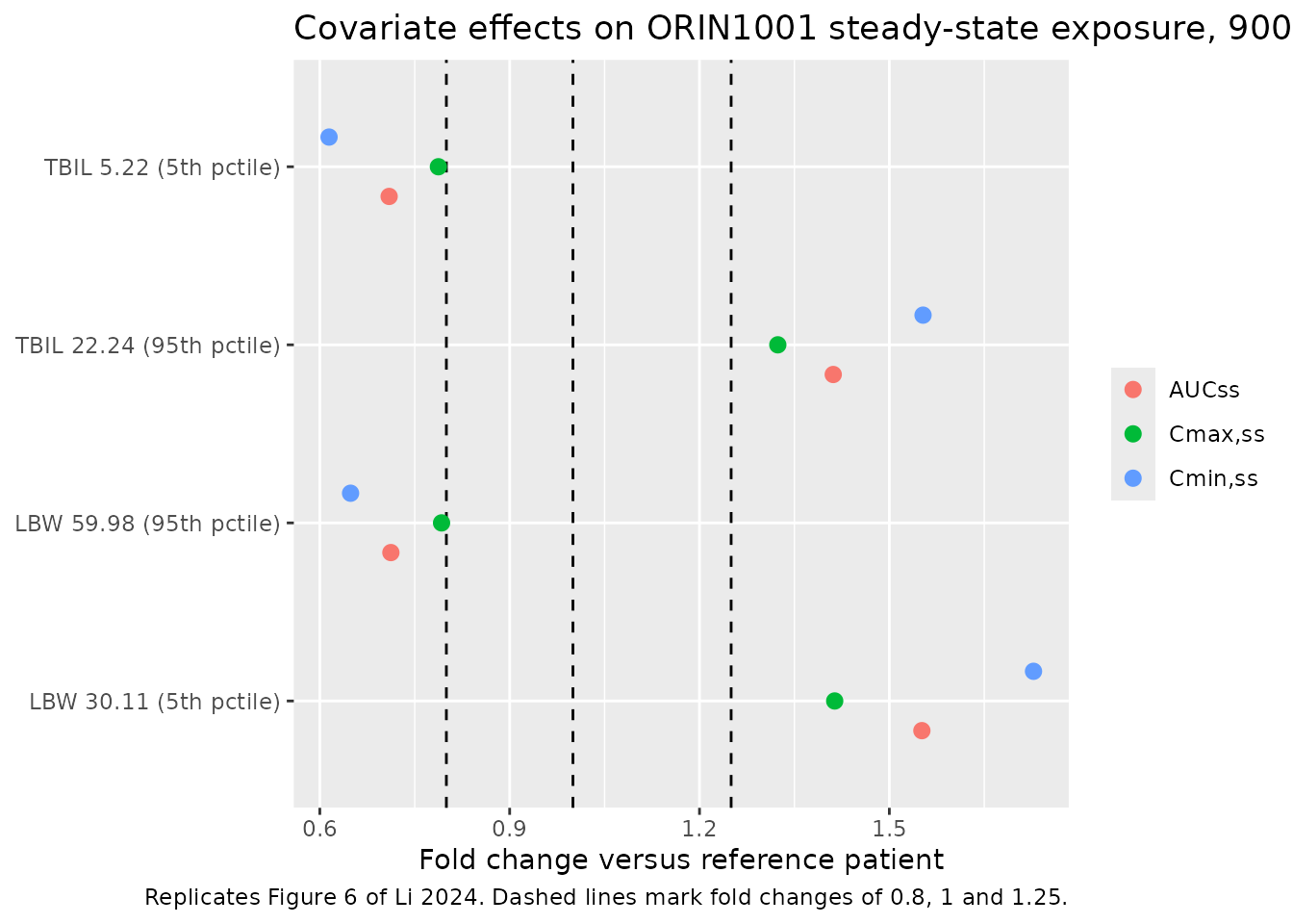
Li 2024 simulated 500 virtual patients per scenario at 900 mg once daily, fixing each significant covariate at its 5th or 95th percentile while holding the others at the cohort median, and reported the mean fold change in steady-state exposure relative to the median-covariate reference patient (Methods 2.6, Results 3.4, Figure 6). Results 3.4 gives four numbers for Cmin,ss, which are the strictest published targets available for this model.
scenarios <- tibble::tribble(
  ~scenario, ~TBILI, ~LBM, ~published_cmin_pct,
  "Reference (LBW 45.13, TBIL 10.3)", 10.30, 45.13, NA,
  "LBW 30.11 (5th pctile)", 10.30, 30.11, 71.8,
  "LBW 59.98 (95th pctile)", 10.30, 59.98, -34.7,
  "TBIL 5.22 (5th pctile)", 5.22, 45.13, -37.4,
  "TBIL 22.24 (95th pctile)", 22.24, 45.13, 58.6
)
n_scen <- 200L # cohort cap; Li 2024 used 500 per scenario

events_scen <- bind_rows(lapply(seq_len(nrow(scenarios)), function(k) {
  s <- tibble(
    id = (k - 1L) * n_scen + seq_len(n_scen),
    scenario = scenarios$scenario[k],
    TBILI = scenarios$TBILI[k], LBM = scenarios$LBM[k], LDH = 214
  )
  bind_rows(
    s |> mutate(time = 0, amt = 900, evid = 1L, cmt = "depot", ii = 24, ss = 1L),
    s |> tidyr::crossing(time = seq(0, 24, by = 0.5)) |>
      mutate(amt = NA_real_, evid = 0L, cmt = "central", ii = 0, ss = 0L)
  )
})) |>
  arrange(id, time, desc(evid))
stopifnot(!anyDuplicated(unique(events_scen[, c("id", "time", "evid")])))

set.seed(1322557)
# steady-state searches for long-half-life subjects exceed the default step budget
sim_scen <- rxode2::rxSolve(mod, events = as.data.frame(events_scen),
                            keep = "scenario", maxsteps = 1e6) |>
  as.data.frame()

per_subject <- sim_scen |>
  filter(!is.na(Cc)) |>
  group_by(scenario, id) |>
  arrange(time, .by_group = TRUE) |>
  summarise(
    Cmax_ss = max(Cc), Cmin_ss = min(Cc),
    AUC_ss = sum(diff(time) * (head(Cc, -1) + tail(Cc, -1)) / 2),
    .groups = "drop"
  )

scen_mean <- per_subject |>
  group_by(scenario) |>
  summarise(across(c(Cmax_ss, Cmin_ss, AUC_ss), mean), .groups = "drop")
ref_row <- scen_mean |> filter(startsWith(scenario, "Reference"))

forest <- scen_mean |>
  mutate(across(c(Cmax_ss, Cmin_ss, AUC_ss),
                ~ .x / ref_row[[cur_column()]][1], .names = "fc_{.col}")) |>
  left_join(scenarios |> select(scenario, published_cmin_pct), by = "scenario") |>
  filter(!startsWith(scenario, "Reference"))

forest |>
  select(scenario, fc_Cmin_ss, fc_Cmax_ss, fc_AUC_ss) |>
  tidyr::pivot_longer(-scenario, names_to = "metric", values_to = "fc") |>
  mutate(metric = recode(metric, fc_Cmin_ss = "Cmin,ss",
                         fc_Cmax_ss = "Cmax,ss", fc_AUC_ss = "AUCss")) |>
  ggplot(aes(fc, scenario, colour = metric)) +
  geom_vline(xintercept = c(0.8, 1, 1.25), linetype = "dashed") +
  geom_point(size = 2.5, position = position_dodge(width = 0.5)) +
  labs(
    x = "Fold change versus reference patient", y = NULL, colour = NULL,
    title = "Covariate effects on ORIN1001 steady-state exposure, 900 mg QD",
    caption = paste(
      "Replicates Figure 6 of Li 2024.",
      "Dashed lines mark fold changes of 0.8, 1 and 1.25."
    )
  )
forest |>
  transmute(
    scenario,
    sim = 100 * (fc_Cmin_ss - 1),
    pub = published_cmin_pct,
    diff_pp = sim - pub,
    cmax = 100 * (fc_Cmax_ss - 1),
    auc = 100 * (fc_AUC_ss - 1)
  ) |>
  dplyr::rename(
    "Scenario" = scenario,
    "Cmin,ss change, simulated (%)" = sim,
    "Cmin,ss change, Li 2024 (%)" = pub,
    "Difference (percentage points)" = diff_pp,
    "Cmax,ss change, simulated (%)" = cmax,
    "AUCss change, simulated (%)" = auc
  ) |>
  knitr::kable(
    digits = 1,
    caption = paste(
      "Steady-state exposure change versus the reference patient.",
      "Published values are from Li 2024 Results 3.4."
    )
)| Scenario | Cmin,ss change, simulated (%) | Cmin,ss change, Li 2024 (%) | Difference (percentage points) | Cmax,ss change, simulated (%) | AUCss change, simulated (%) |
|---|---|---|---|---|---|
| LBW 30.11 (5th pctile) | 72.8 | 71.8 | 1.0 | 41.4 | 55.1 |
| LBW 59.98 (95th pctile) | -35.1 | -34.7 | -0.4 | -20.8 | -28.8 |
| TBIL 22.24 (95th pctile) | 55.3 | 58.6 | -3.3 | 32.4 | 41.1 |
| TBIL 5.22 (5th pctile) | -38.5 | -37.4 | -1.1 | -21.3 | -29.0 |
stopifnot(
  # Every published Cmin,ss change is reproduced within 5 percentage points.
  all(abs(100 * (forest$fc_Cmin_ss - 1) - forest$published_cmin_pct) < 5),
  # Directions match.
  all(sign(forest$fc_Cmin_ss - 1) == sign(forest$published_cmin_pct)),
  # Results 3.4: "The impact of LBW and TBIL on Cmax,ss and AUCss was identified
  # to be similar to that on Cmin,ss, but to a lesser extent."
  all(abs(forest$fc_Cmin_ss - 1) > abs(forest$fc_AUC_ss - 1)),
  all(abs(forest$fc_AUC_ss - 1) > abs(forest$fc_Cmax_ss - 1)),
  # All four scenarios fall outside the paper's 80-125% no-clinical-significance
  # window, which is why Li 2024 called TBIL and LBW clinically significant.
  all(forest$fc_Cmin_ss < 0.8 | forest$fc_Cmin_ss > 1.25)
)
All four published Cmin,ss changes are reproduced to within 3.3 percentage points, and the ordering of sensitivity across the three exposure metrics (Cmin,ss > AUCss > Cmax,ss) matches the paper’s own statement in Results 3.4. Every scenario falls outside the 80-125% window that Li 2024 used as its no-clinical-significance criterion, which is the basis for the paper’s conclusion that total bilirubin and lean body weight are clinically significant covariates.
Assumptions and deviations
- Concentration units. The model returns ug/mL (mg dose / L volume). Li 2024 reports concentrations and AUCs in ng/mL and ng*h/mL; every published value in this vignette has been divided by 1000 to place both on the ug/mL scale. No parameter was rescaled.
- Covariate distributions. Li 2024 publishes the median, IQR, and range for each covariate but not the full distributions or their joint correlation structure. The virtual cohort fits a lognormal to each published median and IQR, evaluates it at deterministic quantiles, and clamps to the published range; the three covariate vectors are rotated relative to each other to give weak cross-correlation, consistent with the paper’s requirement (Methods 2.4.2) that retained covariates have pairwise Pearson correlation below 0.5. The actual pairwise correlations in the trial are shown only graphically (Figure 2) and were not digitised.
- Cohort sizes. 100 participants per dose arm and 200 per covariate scenario, versus Li 2024’s 25 actual subjects and 500 simulated patients per scenario. The reduction is a vignette render-time constraint; the covariate fold changes are stable at this size.
-
Steady state. The multiple-dose period is simulated
with
ss = 1,ii = 24rather than by dosing forward for 21 days. With a terminal half-life near 50 h, day 21 is about ten terminal half-lives and is effectively steady state, and the imposed-steady-state form is the cheaper and less approximation-prone of the two. -
Race and sex are not model covariates. All 25
subjects were Chinese, and neither sex nor race entered the covariate
screen (Methods 2.4.2 lists the candidates); no race or sex distribution
is therefore simulated. Lean body weight is derived from weight, height,
and sex in the source paper via the Janmahasatian formula, so sex enters
only through
LBM. -
Covariate column naming. The model uses the
register canonical names
TBILI,LBM, andLDH. Li 2024’s source columns areTBIL,LBW, andLDH; the first two are recorded assource_nameincovariateData.TBILIis total bilirubin, distinct from the register’sDBIL(direct bilirubin); the paper tabulates total, direct, and indirect bilirubin separately and retained total. Units required no conversion: the paper reports total bilirubin in umol/L, matching the register canonical, and IU/L for LDH, used interchangeably with the canonical U/L. -
Supplementary equations. Equations S1-S3
(
CL2/F,V/F,V2/F) are in Data Sheet 1 of the open-access supplement, which was retrieved and used directly; they are not reproduced in the main text. They are algebraically determined by the general covariate form in Equation 2 together with Table 4, and the supplement confirms them exactly. -
Errata. No erratum or corrigendum for this article
was located. Two transcription hazards in the source are noted rather
than corrected: Table 4 prints the
CL/F95% confidence interval as “0.95 - 11.77”, which is inconsistent with the 5.31% RSE and with the bootstrap interval 0.94-1.18 and is presumably a typesetting error for 1.17 or 1.77; and Supplementary Table S1 prints the base-modelCL/Finterval as “1.00-11.17” in the same way. Neither value is used by this model, which takes only the point estimates. - Not reproduced. Figures 2 (covariate correlation matrix), 3 (individual fits), 5 (NPDE), S3 (goodness-of-fit), and S4 (base-model VPC) depend on the individual observed concentrations, which are not public. Only the final model is packaged; the base model (Supplementary Table S1) is not, as it is superseded within the same paper.