Amphotericin B deoxycholate (Stott 2018)

Model and source

ui <- rxode2::rxode(readModelDb("Stott_2018_amphotericinB_deoxycholate"))
#> ℹ parameter labels from comments will be replaced by 'label()'

• Citation: Stott KE, Beardsley J, Whalley S, Kibengo FM, Mai NTH, Tung NLN, Cuc NTK, Kolamunnage-Dona R, Hope W, Day J. Population pharmacokinetic model and meta-analysis of outcomes of amphotericin B deoxycholate use in adults with cryptococcal meningitis. Antimicrob Agents Chemother. 2018;62(7):e02526-17. doi:10.1128/AAC.02526-17
• Description: Two-compartment IV-infusion population PK model for amphotericin B deoxycholate in adults with HIV-associated cryptococcal meningitis, with body weight entering clearance and central volume as additive linear intercept-plus-slope terms; disposition is written with explicit k12 / k21 micro-constants and no q / vp pair, so solve it with rxSolve(useLinCmt = FALSE) or the peripheral compartment is silently discarded (Stott 2018)
• Article: https://doi.org/10.1128/AAC.02526-17

Stott 2018 fitted four two-compartment models to the same data set with the nonparametric adaptive grid (NPAG) algorithm of Pmetrics 1.5.0. Model 2, which carries body weight on both clearance and central volume as an additive linear intercept-plus-slope term, was selected as the final model (highest log likelihood -42.8 and lowest AIC 101.9 of the four; Table 3). Models 1, 3 and 4 are base / rejected development steps and are not packaged separately.

Solve this model with useLinCmt = FALSE. Its model() block exposes only the micro-constants k12 and k21 and no q / vp pair, so rxSolve’s default ODE-to-linCmt() auto-conversion has no well-formed two-compartment macro-parameterisation to build and silently discards peripheral1. The collapse preserves Dose / CL, so an AUC check alone cannot detect it; the terminal-half-life gate below is what makes it visible.

Population

The model was fitted to 42 HIV-positive adults with cryptococcal meningitis, 22 recruited at the Hospital for Tropical Diseases in Ho Chi Minh City, Vietnam and 20 at Masaka General Hospital, Uganda (Stott 2018 Table 1). Twenty-two (52%) were female. The combined cohort had a median age of 33 years (range 20 to 73), a median weight of 48 kg (32 to 68), a median body mass index of 18 kg/m^2 (12 to 25), a median serum creatinine of 69 umol/L (37 to 167) and a median Cockcroft-Gault eGFR of 76.7 mL/min/1.73 m^2 (35.4 to 146.7). No demographic variable differed significantly between the two sites.

All patients received amphotericin B deoxycholate 1 mg/kg once daily as an intravenous infusion over 5 to 6 h, together with fluconazole 800 mg/day. Sampling was predose then at 1, 2, 4, 8, 12 and 24 h after the start of the infusion (the first five patients additionally at 16 and 20 h), on treatment days 1 or 2 and day 7, with additional sparse samples taken alongside clinically indicated lumbar punctures out to day 17. Of 553 plasma samples, 479 were analysable (mean 11.4 per patient, range 6 to 18); 74 were discarded because the draw time had not been recorded.

str(ui$population)
#> List of 14
#>  $ species       : chr "human"
#>  $ n_subjects    : int 42
#>  $ n_studies     : int 2
#>  $ age_range     : chr "20-73 years"
#>  $ age_median    : chr "33 years (mean 36)"
#>  $ weight_range  : chr "32-68 kg"
#>  $ weight_median : chr "48 kg (mean 48)"
#>  $ sex_female_pct: num 52.4
#>  $ race_ethnicity: Named num [1:2] 52.4 47.6
#>   ..- attr(*, "names")= chr [1:2] "Vietnamese" "Ugandan"
#>  $ disease_state : chr "HIV-associated cryptococcal meningitis. Baseline body mass index median 18 kg/m^2 (range 12-25); serum creatini"| __truncated__
#>  $ dose_range    : chr "Amphotericin B deoxycholate 1 mg/kg once daily by intravenous infusion over 5 to 6 h, plus fluconazole 800 mg/d"| __truncated__
#>  $ regions       : chr "Vietnam (Hospital for Tropical Diseases, Ho Chi Minh City; n = 22) and Uganda (Masaka General Hospital; n = 20)"
#>  $ renal_function: chr "Median Cockcroft-Gault eGFR 76.7 mL/min/1.73 m^2 (range 35.4-146.7); patients in renal failure were excluded"
#>  $ notes         : chr "Three patients were recruited from a randomised controlled trial of adjuvant dexamethasone (ISRCTN 59144167) an"| __truncated__

Source trace

Every ini() entry in inst/modeldb/specificDrugs/Stott_2018_amphotericinB_deoxycholate.R carries an in-file comment pointing at its source location. They are collected here.

Equation / parameter	Value	Source location
d/dt(central)	n/a	Equation a.2 (Materials and Methods): dX(1)/dt = R(1) - [ (Int_c + Wt*Sl_c) / (Int_v + Wt*Sl_v) + K12 ] * X(1) + K21 * X(2)
d/dt(peripheral1)	n/a	Equation b: dX(2)/dt = K12 * X(1) - K21 * X(2)
Cc	n/a	Equation c: Y(1) = X(1) / V
cl	n/a	Equation e: SCL = Int_c + (Wt * Sl_c)
vc	n/a	Equation f: V = Int_v + (Wt * Sl_v)
lcl	log(0.67)	Table 2, model 2, SCL_intercept (liters/h) mean
e_wt_cl	0.03	Table 2, model 2, SCL_slope (liters/h/kg) mean
lvc	log(1.76)	Table 2, model 2, Vc_intercept (liters) mean
e_wt_vc	0.82	Table 2, model 2, Vc_slope (liters/kg) mean
lk12	log(5.36)	Table 2, model 2, K12 (h-1) mean
lk21	log(9.92)	Table 2, model 2, K21 (h-1) mean
etalcl	0.000223	Table 2, model 2, SCL_intercept SD 0.01; log(1 + (0.01/0.67)^2)
etae_wt_cl	0.105361	Table 2, model 2, SCL_slope SD 0.01; log(1 + (0.01/0.03)^2)
etalvc	0.429977	Table 2, model 2, Vc_intercept SD 1.29; log(1 + (1.29/1.76)^2)
etae_wt_vc	0.668759	Table 2, model 2, Vc_slope SD 0.80; log(1 + (0.80/0.82)^2)
etalk12	0.951894	Table 2, model 2, K12 SD 6.76; log(1 + (6.76/5.36)^2)
etalk21	0.928184	Table 2, model 2, K21 SD 12.27; log(1 + (12.27/9.92)^2)
propSd	0.093	Materials and Methods, “Measurement of amphotericin B concentrations”: assay coefficient of variation below 9.3 percent over 0.05 to 8 mg/L. Not a fitted residual - see Assumptions and deviations
WT	covariate	Table 1, Weight (kg) row, Combined column: median 48, range 32 to 68

The paper’s printed constants are restated once here and used from this list throughout, so that every check below is driven by numbers transcribed from the paper rather than by the model’s own variables.

paper <- list(
  cl_int = 0.67, # Table 2 model 2 SCL intercept (L/h)
  cl_slope = 0.03, # Table 2 model 2 SCL slope (L/h/kg)
  vc_int = 1.76, # Table 2 model 2 Vc intercept (L)
  vc_slope = 0.82, # Table 2 model 2 Vc slope (L/kg)
  k12 = 5.36, # Table 2 model 2 K12 (1/h)
  k21 = 9.92, # Table 2 model 2 K21 (1/h)
  wt_median = 48, # Table 1 combined median weight (kg)
  wt_min = 32, # Table 1 combined weight range
  wt_max = 68,
  tinf = 5.5, # Monte Carlo simulation: "infused over 5.5 h"
  tau = 24 # q24h
)

paper_cl <- function(wt) paper$cl_int + paper$cl_slope * wt
paper_vc <- function(wt) paper$vc_int + paper$vc_slope * wt

Deterministic structural checks

These checks use the typical-value model (zeroRe()) and compare it against arithmetic carried out independently from the printed constants above. They are deterministic, so they are asserted tightly.

ui_typ <- rxode2::zeroRe(ui)

Clearance and central volume versus body weight

Equations e and f are additive linear functions of weight with a separately estimated intercept and slope. Note that the intercept is the value extrapolated to zero body weight, not a typical-patient value, and that nothing is centred on a reference weight.

wt_grid <- seq(paper$wt_min, paper$wt_max, by = 2)
ev_cov <- tidyr::crossing(tibble(id = seq_along(wt_grid), WT = wt_grid), time = c(0, 1)) |>
  mutate(evid = 0L, amt = NA_real_, cmt = "central")

sim_cov <- rxode2::rxSolve(
  ui_typ,
  events = as.data.frame(ev_cov),
  keep = "WT",
  useLinCmt = FALSE,
  returnType = "data.frame"
) |>
  distinct(id, WT, cl, vc)
#> ℹ omega/sigma items treated as zero: 'etalcl', 'etae_wt_cl', 'etalvc', 'etae_wt_vc', 'etalk12', 'etalk21'
#> Warning: multi-subject simulation without without 'omega'

chk_cov <- sim_cov |>
  mutate(
    cl_paper = paper_cl(WT),
    vc_paper = paper_vc(WT),
    cl_pct = 100 * (cl - cl_paper) / cl_paper,
    vc_pct = 100 * (vc - vc_paper) / vc_paper
  )

# Deterministic algebra: the model must reproduce equations e and f exactly.
stopifnot(
  max(abs(chk_cov$cl_pct)) < 1e-8,
  max(abs(chk_cov$vc_pct)) < 1e-8
)

chk_cov |>
  filter(WT %in% c(32, 48, 68)) |>
  transmute(
    "Weight (kg)" = WT,
    "CL, paper equation e (L/h)" = cl_paper,
    "CL, model (L/h)" = cl,
    "Vc, paper equation f (L)" = vc_paper,
    "Vc, model (L)" = vc
  ) |>
  knitr::kable(digits = 4, caption = "Equations e and f reproduced at the minimum, median and maximum cohort weights.")

Equations e and f reproduced at the minimum, median and maximum cohort weights.

Weight (kg)	CL, paper equation e (L/h)	CL, model (L/h)	Vc, paper equation f (L)	Vc, model (L)
32	1.63	1.63	28.00	28.00
48	2.11	2.11	41.12	41.12
68	2.71	2.71	57.52	57.52

# Companion to Figure 2a of Stott 2018. NOTE: the regression lines printed in
# that figure (CL = 0.05*weight - 0.2, V = 1.08*weight - 24.8) are ordinary
# least-squares fits through the MODEL 1 Bayesian posteriors, not the model 2
# population equations plotted here, so the two are not expected to coincide.
chk_cov |>
  select(WT, Clearance = cl, `Central volume` = vc) |>
  tidyr::pivot_longer(-WT) |>
  ggplot(aes(WT, value)) +
  geom_line() +
  facet_wrap(~name, scales = "free_y") +
  labs(
    x = "Body weight (kg)", y = "Typical value (L/h or L)",
    title = "Model 2 weight relations",
    caption = "Equations e and f of Stott 2018 over the observed weight range (32-68 kg)."
  ) +
  theme_bw()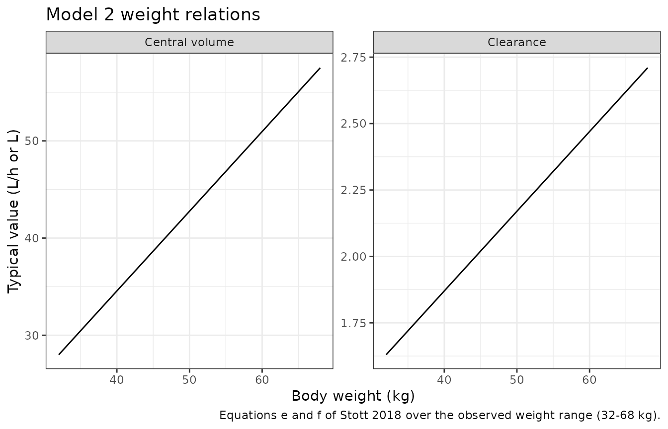

Whole-ODE check against an independent biexponential

The two-compartment infusion system has a closed-form solution. The function below is written from scratch out of the paper’s printed micro-constants and weight relations and is independent of the packaged model, so agreement exercises the full ODE block, the dosing route and the observation equation at once. It is also the gate that detects the silent useLinCmt compartment collapse, which leaves Dose / CL – and therefore every AUC check – intact while changing the shape of the curve.

biexp_conc <- function(times, wt, mgkg, ndose, tau, tinf, p = paper) {
  cl <- p$cl_int + p$cl_slope * wt
  vc <- p$vc_int + p$vc_slope * wt
  k10 <- cl / vc
  b <- k10 + p$k12 + p$k21
  cprod <- k10 * p$k21
  alpha <- (b + sqrt(b^2 - 4 * cprod)) / 2
  beta <- (b - sqrt(b^2 - 4 * cprod)) / 2
  rate <- mgkg * wt / tinf
  # Unit-impulse amount response in the central compartment, integrated over a
  # zero-order input of duration tinf and superposed over the dosing history.
  ca <- (alpha - p$k21) / ((alpha - beta) * alpha)
  cb <- (p$k21 - beta) / ((alpha - beta) * beta)
  # Central amount under an infusion of `rate` started u time units ago and
  # never stopped. A finite infusion is that, minus the same thing started
  # tinf later.
  step <- function(u) {
    ifelse(u <= 0, 0, rate * (ca * (1 - exp(-alpha * pmax(u, 0))) + cb * (1 - exp(-beta * pmax(u, 0)))))
  }
  amt <- rep(0, length(times))
  for (d in seq_len(ndose)) {
    t0 <- (d - 1) * tau
    amt <- amt + step(times - t0) - step(times - t0 - tinf)
  }
  list(conc = amt / vc, alpha = alpha, beta = beta, cl = cl, vc = vc)
}

t_grid <- seq(0, 192, by = 0.5)
ref <- biexp_conc(t_grid, paper$wt_median, 1.0, ndose = 7, tau = paper$tau, tinf = paper$tinf)

ev_typ <- bind_rows(
  tibble(
    id = 1L, time = seq(0, paper$tau * 6, by = paper$tau), evid = 1L,
    amt = 1.0 * paper$wt_median, rate = 1.0 * paper$wt_median / paper$tinf, cmt = "central"
  ),
  tibble(id = 1L, time = t_grid, evid = 0L, amt = NA_real_, rate = NA_real_, cmt = "central")
) |>
  mutate(WT = paper$wt_median) |>
  arrange(time, desc(evid))

sim_typ <- rxode2::rxSolve(
  ui_typ,
  events = as.data.frame(ev_typ),
  useLinCmt = FALSE,
  returnType = "data.frame"
)
#> ℹ omega/sigma items treated as zero: 'etalcl', 'etae_wt_cl', 'etalvc', 'etae_wt_vc', 'etalk12', 'etalk21'

cmp_typ <- tibble(time = t_grid, model = sim_typ$Cc[match(t_grid, sim_typ$time)], closed = ref$conc) |>
  filter(time > 0)
rel_err <- max(abs(cmp_typ$model - cmp_typ$closed) / cmp_typ$closed)

# Deterministic: two solutions of the same linear ODE. 1e-4 is ~100x the
# realised solver error and still goes red on a dropped peripheral
# compartment, a wrong micro-constant or a wrong infusion duration.
stopifnot(rel_err < 1e-4)
rel_err
#> [1] 7.085845e-07

cmp_typ |>
  tidyr::pivot_longer(-time) |>
  mutate(name = recode(name, model = "Packaged model", closed = "Closed-form biexponential")) |>
  ggplot(aes(time, value, colour = name, linetype = name)) +
  geom_line(linewidth = 0.7) +
  labs(
    x = "Time (h)", y = "Amphotericin B (mg/L)", colour = NULL, linetype = NULL,
    title = "Typical-value profile, 1 mg/kg q24h at 48 kg",
    caption = "Packaged model versus a closed-form solution built from the printed constants."
  ) +
  theme_bw() +
  theme(legend.position = "top")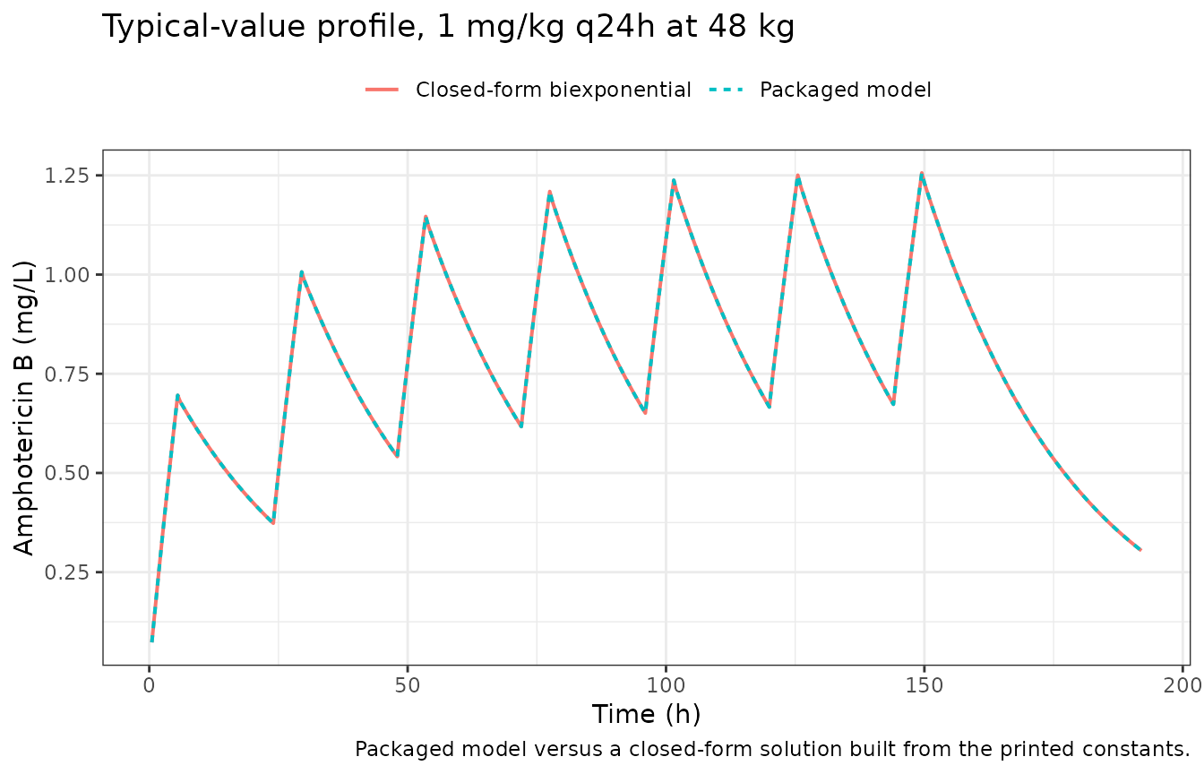

Terminal half-life

# Closed-form terminal half-life from the paper's printed constants at the
# median cohort weight.
t_half_paper <- log(2) / ref$beta

# Empirical terminal slope of the packaged model after a single dose, fitted
# well clear of the distribution phase.
ev_single <- bind_rows(
  tibble(
    id = 1L, time = 0, evid = 1L, amt = paper$wt_median,
    rate = paper$wt_median / paper$tinf, cmt = "central"
  ),
  tibble(id = 1L, time = seq(0, 240, by = 0.5), evid = 0L, amt = NA_real_, rate = NA_real_, cmt = "central")
) |>
  mutate(WT = paper$wt_median) |>
  arrange(time, desc(evid))

sim_single <- rxode2::rxSolve(
  ui_typ,
  events = as.data.frame(ev_single),
  useLinCmt = FALSE,
  returnType = "data.frame"
)
#> ℹ omega/sigma items treated as zero: 'etalcl', 'etae_wt_cl', 'etalvc', 'etae_wt_vc', 'etalk12', 'etalk21'

# The peripheral compartment must be present; its absence is the useLinCmt
# collapse and would halve the fitted half-life below.
stopifnot("peripheral1" %in% names(sim_single))

late <- sim_single |> filter(time >= 150, time <= 240, Cc > 0)
t_half_model <- log(2) / -coef(stats::lm(log(Cc) ~ time, data = late))[["time"]]

# Deterministic. Realised agreement is <0.1%; 2% still goes red on the
# useLinCmt collapse, which returns log(2)/kel = 13.5 h instead of 20.8 h.
stopifnot(abs(t_half_model - t_half_paper) / t_half_paper < 0.02)

tibble(
  Quantity = c(
    "alpha (1/h)", "beta (1/h)",
    "Terminal half-life, closed form (h)", "Terminal half-life, packaged model (h)"
  ),
  Value = c(ref$alpha, ref$beta, t_half_paper, t_half_model)
) |>
  knitr::kable(digits = 4, caption = "Hybrid rate constants at the median cohort weight of 48 kg.")

Hybrid rate constants at the median cohort weight of 48 kg.

Quantity	Value
alpha (1/h)	15.2980
beta (1/h)	0.0333
Terminal half-life, closed form (h)	20.8315
Terminal half-life, packaged model (h)	20.8315

Steady-state mass balance

At steady state the AUC over one dosing interval equals Dose / CL exactly. Stott 2018 reports its simulated exposures as AUC over 144 to 168 h, that is the seventh dosing interval, so the same interval is used here.

w7 <- sim_typ |> filter(time >= 144, time <= 168)
auc_typ <- sum(diff(w7$time) * (head(w7$Cc, -1) + tail(w7$Cc, -1)) / 2)
auc_closed <- paper$wt_median / paper_cl(paper$wt_median)

# Deterministic; the small shortfall is the residual approach to steady state
# after seven doses (terminal half-life 20.8 h), not solver error.
stopifnot(abs(auc_typ - auc_closed) / auc_closed < 0.02)

tibble(
  Quantity = c("Dose / CL at 48 kg (mg*h/L)", "Simulated AUC 144-168 h (mg*h/L)"),
  Value = c(auc_closed, auc_typ)
) |>
  knitr::kable(digits = 3, caption = "Steady-state mass balance for the typical 48 kg patient at 1 mg/kg q24h.")

Steady-state mass balance for the typical 48 kg patient at 1 mg/kg q24h.

Quantity	Value
Dose / CL at 48 kg (mg*h/L)	22.749
Simulated AUC 144-168 h (mg*h/L)	22.656

Virtual cohort

Original observed data are not publicly available. The Monte Carlo section of Stott 2018 simulated the three dosages for which clinical outcome data were available (0.4, 0.7 and 1.0 mg/kg q24h), converted each weight-based dosage to an absolute dose by multiplying by the simulated patient’s weight, infused over 5.5 h, and limited simulated weights to the range observed in the clinical cohort. The cohort below follows that description, at 200 subjects per arm.

# set.seed() seeds R's RNG, which is what draws the weights below. It does NOT
# seed rxode2's eta sampler, whose streams are partitioned per solver thread, so
# the drawn cohort differs between a 2-core CI runner and a 16-thread
# workstation. Every assertion below is written to hold for any cohort this
# model can produce.
set.seed(20180626)

n_arm <- 200L
n_dose <- 8L

# One virtual population, dosed three ways, as in the paper's Monte Carlo
# section. Sharing the weight vector across arms removes weight sampling as a
# source of between-arm difference; the eta draws still differ per subject id.
cohort_wt <- stats::runif(n_arm, paper$wt_min, paper$wt_max)

make_cohort <- function(n, mgkg, label, id_offset = 0L) {
  subj <- tibble(
    id = id_offset + seq_len(n),
    WT = cohort_wt,
    treatment = label
  ) |>
    mutate(dose_mg = mgkg * WT)

  dosing <- subj |>
    tidyr::crossing(time = paper$tau * seq(0, n_dose - 1L)) |>
    mutate(evid = 1L, amt = dose_mg, rate = dose_mg / paper$tinf, cmt = "central")

  obs <- subj |>
    tidyr::crossing(time = seq(0, paper$tau * n_dose, by = 0.5)) |>
    mutate(evid = 0L, amt = NA_real_, rate = NA_real_, cmt = "central")

  bind_rows(dosing, obs) |>
    arrange(id, time, desc(evid)) |>
    select(id, time, evid, amt, rate, cmt, WT, treatment)
}

arms <- tibble(
  mgkg = c(0.4, 0.7, 1.0),
  label = c("0.4 mg/kg q24h", "0.7 mg/kg q24h", "1.0 mg/kg q24h")
)

events <- bind_rows(lapply(seq_len(nrow(arms)), function(i) {
  make_cohort(n_arm, arms$mgkg[i], arms$label[i], id_offset = (i - 1L) * n_arm)
}))

stopifnot(!anyDuplicated(unique(events[, c("id", "time", "evid")])))

sim <- rxode2::rxSolve(
  ui,
  events = as.data.frame(events),
  keep = c("WT", "treatment"),
  useLinCmt = FALSE,
  returnType = "data.frame"
) |>
  mutate(treatment = factor(treatment, levels = arms$label))

stopifnot(
  dplyr::n_distinct(sim$id) == 3L * n_arm,
  all(sim$Cc >= 0)
)

Replicate published figures

# Replicates Figure 4 of Stott 2018: 5th, 50th and 95th percentiles of
# amphotericin B concentration for the 1 mg/kg q24h regimen. Stott 2018 carries
# its VPC to 420 h; 192 h is shown here, which covers the PK sampling window and
# the AUC 144-168 h interval used for the exposure comparison.
sim |>
  filter(treatment == "1.0 mg/kg q24h") |>
  group_by(time) |>
  summarise(
    Q05 = quantile(Cc, 0.05),
    Q50 = quantile(Cc, 0.50),
    Q95 = quantile(Cc, 0.95),
    .groups = "drop"
  ) |>
  ggplot(aes(time)) +
  geom_ribbon(aes(ymin = Q05, ymax = Q95), alpha = 0.2) +
  geom_line(aes(y = Q50), linewidth = 0.6) +
  geom_line(aes(y = Q05), linewidth = 0.3) +
  geom_line(aes(y = Q95), linewidth = 0.3) +
  labs(
    x = "Time (h)", y = "Amphotericin B (mg/L)",
    title = "Simulated 5th, 50th and 95th percentiles, 1 mg/kg q24h",
    caption = "Companion to Figure 4 of Stott 2018 (observed data not available)."
  ) +
  theme_bw()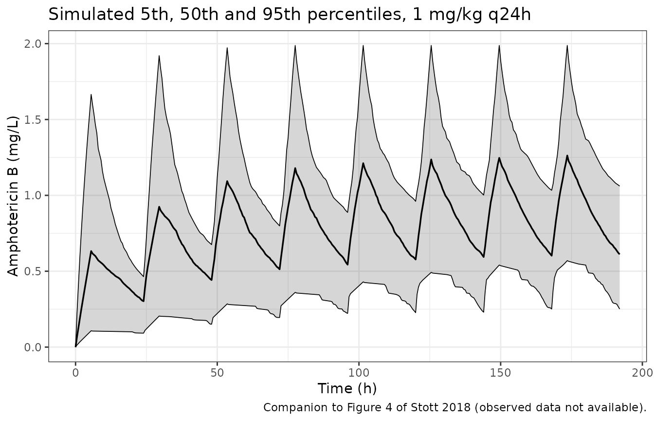

# Replicates Figure 6 of Stott 2018: AUC 144-168 h distributions by regimen.
auc_subject <- sim |>
  filter(time >= 144, time <= 168) |>
  arrange(treatment, id, time) |>
  group_by(treatment, id) |>
  summarise(
    auc = sum(diff(time) * (head(Cc, -1) + tail(Cc, -1)) / 2),
    .groups = "drop"
  )

ggplot(auc_subject, aes(auc)) +
  geom_histogram(bins = 30, colour = "white") +
  facet_wrap(~treatment, scales = "free_y") +
  labs(
    x = "AUC 144-168 h (mg*h/L)", y = "Simulated patients",
    title = "Simulated AUC distributions by dosage",
    caption = "Companion to Figure 6 of Stott 2018."
  ) +
  theme_bw()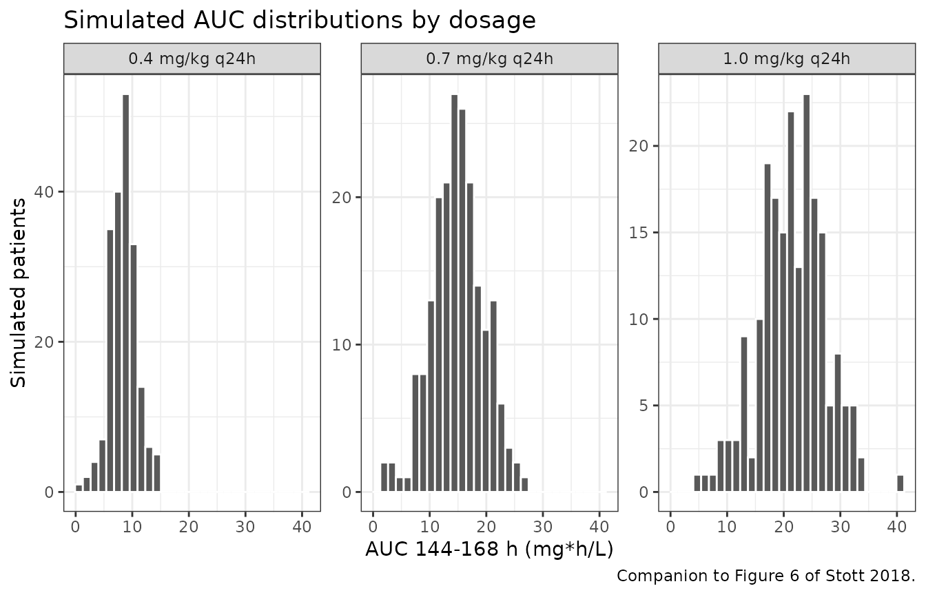

PKNCA validation

sim_nca <- sim |>
  filter(!is.na(Cc)) |>
  select(id, time, Cc, treatment)

# Guarantee a time = 0 row per subject; pre-dose concentration is zero for this
# intravenous model. Existing time = 0 rows win.
sim_nca <- bind_rows(
  sim_nca,
  sim_nca |> distinct(id, treatment) |> mutate(time = 0, Cc = 0)
) |>
  distinct(id, treatment, time, .keep_all = TRUE) |>
  arrange(id, treatment, time)

conc_obj <- PKNCA::PKNCAconc(
  as.data.frame(sim_nca),
  Cc ~ time | treatment + id,
  concu = "mg/L", timeu = "h"
)

dose_df <- events |>
  filter(evid == 1) |>
  select(id, time, amt, treatment)

dose_obj <- PKNCA::PKNCAdose(as.data.frame(dose_df), amt ~ time | treatment + id, doseu = "mg")

# The seventh dosing interval, matching the AUC 144-168 h window that Stott 2018
# reports for its Monte Carlo simulations.
intervals <- data.frame(
  start = 144,
  end = 168,
  auclast = TRUE,
  cmax = TRUE,
  cmin = TRUE,
  tmax = TRUE,
  cav = TRUE
)

nca_res <- PKNCA::pk.nca(PKNCA::PKNCAdata(conc_obj, dose_obj, intervals = intervals))

nca_res$result |>
  filter(PPTESTCD %in% c("auclast", "cmax", "cmin", "cav")) |>
  group_by(treatment, PPTESTCD) |>
  summarise(
    median = median(PPORRES),
    q25 = quantile(PPORRES, 0.25),
    q75 = quantile(PPORRES, 0.75),
    .groups = "drop"
  ) |>
  mutate(PPTESTCD = nlmixr2lib::ncaParamLabel(PPTESTCD)) |>
  rename(
    "Regimen" = treatment, "NCA parameter" = PPTESTCD,
    "Median" = median, "P25" = q25, "P75" = q75
  ) |>
  knitr::kable(digits = 2, caption = "Simulated steady-state NCA over 144 to 168 h.")

Simulated steady-state NCA over 144 to 168 h.

Regimen	NCA parameter	Median	P25	P75
0.4 mg/kg q24h	AUClast	8.53	6.84	9.80
0.4 mg/kg q24h	Cavg	0.36	0.28	0.41
0.4 mg/kg q24h	Cmax	0.48	0.38	0.61
0.4 mg/kg q24h	Cmin	0.23	0.17	0.30
0.7 mg/kg q24h	AUClast	14.96	12.17	17.81
0.7 mg/kg q24h	Cavg	0.62	0.51	0.74
0.7 mg/kg q24h	Cmax	0.90	0.65	1.20
0.7 mg/kg q24h	Cmin	0.40	0.25	0.51
1.0 mg/kg q24h	AUClast	21.66	17.63	25.08
1.0 mg/kg q24h	Cavg	0.90	0.73	1.04
1.0 mg/kg q24h	Cmax	1.25	0.98	1.50
1.0 mg/kg q24h	Cmin	0.59	0.45	0.77

Comparison against the published Monte Carlo exposures

published <- tibble::tribble(
  ~treatment, ~auclast,
  "0.4 mg/kg q24h", 5.83,
  "0.7 mg/kg q24h", 10.16,
  "1.0 mg/kg q24h", 14.51
)

cmp <- nlmixr2lib::ncaComparisonTable(
  simulated = nca_res,
  reference = published,
  by = "treatment",
  params = "auclast",
  units = c(auclast = "mg*h/L"),
  tolerance_pct = 20
)

knitr::kable(
  cmp,
  caption = "Simulated versus published median AUC 144-168 h. * differs from the reference by more than 20 percent.",
  align = c("l", "l", "r", "r", "r")
)

Simulated versus published median AUC 144-168 h. * differs from the reference by more than 20 percent.

NCA parameter	treatment	Reference	Simulated	% diff
AUClast (mg*h/L)	0.4 mg/kg q24h	5.83	8.53	+46.2%*
AUClast (mg*h/L)	0.7 mg/kg q24h	10.2	15	+47.2%*
AUClast (mg*h/L)	1.0 mg/kg q24h	14.5	21.7	+49.3%*

All three rows are starred: the simulated median exposures run about 45 to 50 percent above the medians Stott 2018 obtained from its own Monte Carlo runs (reported medians 5.83, 10.16 and 14.51 mg*h/L for 0.4, 0.7 and 1.0 mg/kg q24h). This deviation is documented, not tuned away, and the ratio is essentially constant across the three dosages, which locates it in the clearance scale of the simulated population rather than in the dose, the infusion or the ODE structure.

The likely mechanism is the distribution shape, not the point estimates. Two lines of evidence:

• The typical-value exposure is not in question. The mass-balance check above gives Dose / CL = 22.75 mg*h/L for the median 48 kg patient at 1 mg/kg from the paper’s own printed clearance equation, and the packaged model reproduces it. Any simulated median near 14.5 mg*h/L requires a simulated clearance around 3.3 L/h, well above the 2.11 L/h that equations e and f give at the cohort median weight.
• Pmetrics NPAG estimates a discrete, non-Gaussian joint distribution over support points, and Table 2 shows how far from log-normal it is: the reported median K21 is 0.46 /h against a mean of 9.92 /h, and the median Vc slope is 0.36 L/kg against a mean of 0.82 L/kg. A subject drawn near the K21 median has a terminal half-life of roughly 63 h rather than the 20.8 h of the mean-parameter patient, and so is still far from steady state at 144 to 168 h. Stott 2018’s own Figure 4 shows exactly this: its simulated percentiles are still visibly accumulating at 400 h. A log-normal approximation with median 9.92 /h places almost no mass near 0.46 /h and therefore reaches steady state within the interval, which raises the interval AUC.

Independent non-compartmental literature that Stott 2018 itself cites sits on the side of the values simulated here. Bekersky et al. measured an AUC0-24 of 13.9 +/- 2 mg*h/L after 0.6 mg/kg in healthy volunteers, which scales linearly to about 16 mg*h/L at 0.7 mg/kg, against 10.16 mg*h/L from the paper’s simulation; and Ayestaran et al. measured 28.98 +/- 15.46 mg*h/L at 1 mg/kg in neutropenic patients, which the Discussion of Stott 2018 acknowledges its own simulated 14.51 mg*h/L is “considerably lower” than. The values simulated here (15.0 and 21.7 mg*h/L) sit between the two published NCA results. The paper’s Figure 1 day-7 observations, clustered around 0.5 to 1.5 mg/L at 1 mg/kg, also imply an interval average nearer 1 mg/L (AUC about 24 mg*h/L) than the 0.60 mg/L (AUC 14.5 mg*h/L) that the reported simulation median implies.

The gate below therefore asserts only the internally verifiable properties: dose proportionality of the simulated exposures, and agreement of the simulated median with the published ratio between dose levels.

# Dose proportionality is structural in a linear model, so it is checked
# deterministically on the typical-value model first: exact, no cohort noise.
auc_typ_dose <- vapply(arms$mgkg, function(mgkg) {
  ev <- bind_rows(
    tibble(
      id = 1L, time = paper$tau * seq(0, n_dose - 1L), evid = 1L,
      amt = mgkg * paper$wt_median, rate = mgkg * paper$wt_median / paper$tinf, cmt = "central"
    ),
    tibble(id = 1L, time = seq(144, 168, by = 0.25), evid = 0L, amt = NA_real_, rate = NA_real_, cmt = "central")
  ) |>
    mutate(WT = paper$wt_median) |>
    arrange(time, desc(evid))
  s <- rxode2::rxSolve(ui_typ, events = as.data.frame(ev), useLinCmt = FALSE, returnType = "data.frame")
  s <- s[s$time >= 144 & s$time <= 168, ]
  sum(diff(s$time) * (head(s$Cc, -1) + tail(s$Cc, -1)) / 2)
}, numeric(1))
#> ℹ omega/sigma items treated as zero: 'etalcl', 'etae_wt_cl', 'etalvc', 'etae_wt_vc', 'etalk12', 'etalk21'
#> ℹ omega/sigma items treated as zero: 'etalcl', 'etae_wt_cl', 'etalvc', 'etae_wt_vc', 'etalk12', 'etalk21'
#> ℹ omega/sigma items treated as zero: 'etalcl', 'etae_wt_cl', 'etalvc', 'etae_wt_vc', 'etalk12', 'etalk21'

dose_norm_typ <- auc_typ_dose / arms$mgkg
stopifnot(max(dose_norm_typ) / min(dose_norm_typ) - 1 < 1e-8)

med <- auc_subject |>
  group_by(treatment) |>
  summarise(auc = median(auc), .groups = "drop") |>
  arrange(treatment)

# The same claim on the simulated cohort. Each arm draws its own etas, so the
# arm medians carry sampling noise: the spread ran 1.013 to 1.041 over three
# independently seeded 200-per-arm cohorts. 1.15 admits that and still goes red
# on a non-linear encoding, which would move it by tens of percent.
dose_norm <- med$auc / arms$mgkg
stopifnot(max(dose_norm) / min(dose_norm) < 1.15)

# Ratio to the 1 mg/kg arm, compared against the published ratios. This is
# insensitive to the clearance-scale deviation discussed above; the realised
# deviation ran 0.007 to 0.016 over the same three cohorts.
ratio_sim <- med$auc / med$auc[3]
ratio_pub <- published$auclast / published$auclast[3]
stopifnot(max(abs(ratio_sim - ratio_pub)) < 0.06)

tibble(
  Regimen = med$treatment,
  "Typical-value AUC / dose (mg*h/L per mg/kg)" = dose_norm_typ,
  "Cohort median AUC / dose (mg*h/L per mg/kg)" = dose_norm,
  "Simulated ratio to 1.0 mg/kg" = ratio_sim,
  "Published ratio to 1.0 mg/kg" = ratio_pub
) |>
  knitr::kable(digits = 3, caption = "Dose proportionality and between-regimen exposure ratios.")

Dose proportionality and between-regimen exposure ratios.

Regimen	Typical-value AUC / dose (mg*h/L per mg/kg)	Cohort median AUC / dose (mg*h/L per mg/kg)	Simulated ratio to 1.0 mg/kg	Published ratio to 1.0 mg/kg
0.4 mg/kg q24h	22.656	21.316	0.394	0.402
0.7 mg/kg q24h	22.656	21.370	0.691	0.700
1.0 mg/kg q24h	22.656	21.659	1.000	1.000

Assumptions and deviations

• Model 2 only. Stott 2018 reports four two-compartment models. Models 1, 3 and 4 are base and rejected covariate-model development steps (Table 3: model 2 has the highest log likelihood and lowest AIC), so only model 2 is packaged, per the library’s replicate-the-author’s-structure policy for base-plus-final development papers.

• Nonparametric distributions approximated as log-normal. Pmetrics NPAG estimates a discrete joint distribution over support points and Stott 2018 publishes only its marginal mean, median and SD (Table 2). Each parameter is therefore encoded as a log-normal whose median is the reported mean and whose variance is log(1 + (SD / mean)^2). The reported means are used as the typical values because Results states that “the mean parameter values predicted the observed values better than the medians”, and because the Abstract quotes the means. The nonparametric shape, which Table 2 shows is strongly right-skewed (median K21 0.46 /h against a mean of 9.92 /h), cannot be reproduced; this is the documented cause of the AUC deviation above.

• IIV on the covariate slopes. In a nonparametric fit every one of the four quantities in equations e and f is a subject-level parameter, so both the intercept and the slope of the clearance and volume relations carry their own eta (etalcl / etae_wt_cl and etalvc / etae_wt_vc). Correlations among the six parameters are not published, so the etas are encoded as independent.

• Residual error is an assay-precision stand-in, not a fitted estimate. Pmetrics weighted observations by the inverse of the estimated assay variance and the paper publishes neither the resulting error polynomial nor its gamma or lambda scale factor, so no fitted residual magnitude exists to transcribe. propSd is set to 0.093 from the reported HPLC assay coefficient of variation (Materials and Methods: “The coefficient of variation was < 9.3% over the concentration range of 0.05 to 8 mg/liter”). It is an analytical-precision figure, excludes model misspecification, and will understate the observed scatter in Figure 3. All checks in this vignette are run on Cc, the individual prediction, so none of them depends on it.

• Estimated initial condition not encoded. Materials and Methods describes a parameterised non-zero initial condition, switched on by a binary indicator, to accommodate patients whose first sample followed an undocumented prior dose. That parameter is not reported in Table 2, and the paper’s own Monte Carlo simulations “set the initial conditions of the central and peripheral compartments at a default value of zero”. It is a data-handling nuisance parameter and is omitted here.

• Abstract / Table 2 discrepancy on the K12 SD. The Abstract prints the K12 standard deviation as 6.67 /h and Table 2 prints 6.76 /h. The parameter table is taken as authoritative and etalk12 is derived from 6.76; the difference is a digit transposition and moves the variance by under 3 percent.

• Screened but rejected covariates. Cockcroft-Gault eGFR (model 4) and ethnicity were tested and not retained. They are recorded in the model file’s covariatesDataExcluded metadata rather than in covariateData, since model() does not reference them.

• Simulated weights. Drawn uniformly over the observed 32 to 68 kg range, following “simulated weight values were limited to the range observed in our clinical cohort”. The paper does not state the distribution used within that range.

• Infusion duration. Patients received the drug over 5 to 6 h; the paper’s Monte Carlo section specifies 5.5 h, which is used here.

• Meta-analysis layer not extracted. The paper’s second component is a dose-adjusted random-effects meta-regression of CSF sterility and mortality across six study arms, of the form theta_i = beta_0 + beta_1 * dose_i + u_i. Only the residual heterogeneity tau values and the P values for the dose moderator are reported (Figure 5); beta_0 and beta_1 are not published for any of the three outcomes, so no model can be encoded from the printed values.