Model and source
- Citation: Liao M, Zhou J, Wride K, Lepley D, Cameron T, Sale M, Xiao J. (2022). Population Pharmacokinetic Modeling of Lucitanib in Patients with Advanced Cancer. European Journal of Drug Metabolism and Pharmacokinetics 47(5):711-723. doi:10.1007/s13318-022-00773-w.
- Description: Two-compartment population PK model for oral lucitanib (a VEGFR1-3 / FGFR1-3 / PDGFRalpha/beta tyrosine kinase inhibitor) in 403 adults with advanced cancers pooled from five phase 1/2 studies (Liao 2022). Absorption is sequential: a zero-order release of duration D1 into the depot followed by first-order absorption (ka) into the central compartment; elimination is linear from central. D1 is 0.814 h for the hard gelatin capsule and 0.299-fold shorter (0.243 h) for the film-coated tablet. CL/F and Q/F scale with (WT/70)^0.75 and Vc/F and Vp/F with (WT/70)^1 (exponents fixed). IIV on CL/F and Vc/F (correlated), D1 and Vp/F; proportional residual error.
- Article: https://doi.org/10.1007/s13318-022-00773-w (open access)
- Supplement: Electronic Supplementary Material 1 of the article (Supplemental Table 1, Figures S1-S5 and the NONMEM control stream of the final model).
Population
Liao 2022 pooled 3540 lucitanib plasma concentrations from 403 adults with advanced cancers enrolled in five phase 1/2 studies (Table 1): the first-in-human dose-escalation and expansion study E-3810-I-01 (n = 134, advanced solid tumours), the phase 2 breast-cancer studies CO-3810-025 (n = 164) and FINESSE (n = 72), the phase 1b INES study combining lucitanib with fulvestrant (n = 17), and the phase 2 lung-cancer study E3810-II-02 (n = 16). Lucitanib was given orally at 5-30 mg once daily, continuously or 15 mg on 5/2 or 21/7 day schedules, as a film-coated tablet or a hard gelatin capsule. Table 3 gives a median age of 55 years (range 26-82), a median body weight of 67.5 kg (35.9-159), 82% women (332/403), and 84% White, 4% Black, 2.5% Asian and 9% other race. Median creatinine clearance was 95.1 mL/min; 141 patients had mild and 40 moderate renal impairment, and 80 mild hepatic impairment.
The same information is available programmatically via
readModelDb("Liao_2022_lucitanib")()$population.
Source trace
Every ini() value carries its source in an in-file
comment in
inst/modeldb/specificDrugs/Liao_2022_lucitanib.R. The
structural equations come from the NONMEM control stream of the final
model in the Supplemental File ($SUBROUTINES ADVAN4 TRANS4,
$PK, $ERROR).
| Equation / parameter | Value | Source location |
|---|---|---|
lcl (CL/F, 70 kg) |
log(1.90) L/h | Table 4 |
lvc (Vc/F, 70 kg) |
log(63.8) L | Table 4 |
lka (ka) |
log(4.86) 1/h | Table 4 |
lq (Q/F, 70 kg) |
log(6.23) L/h | Table 4 |
lvp (Vp/F, 70 kg) |
log(69.1) L | Table 4 |
ld1 (D1, capsule) |
log(0.814) h | Table 4 |
e_form_tablet_d1 |
0.299 | Table 4 ‘Effect of formulation on D1 (tablet to capsule ratio)’;
control stream TVD1 = THETA(8)*THETA(10)**FORM
|
e_wt_cl |
0.75 (fixed) | Section 2.2; Table 4; control stream (WT/70)**0.75 on
CL and Q |
e_wt_vc |
1 (fixed) | Section 2.2; Table 4; control stream (WT/70) on V2 and
V3 |
etalcl, etalvc, covariance |
0.2058, 0.2952, 0.1469 | Table 4 BSV 47.8% and 58.6%, correlation 0.596;
$OMEGA BLOCK(2)
|
etald1 |
0.3084 | Table 4 BSV 60.1% |
etalvp |
0.4627 | Table 4 BSV 76.7% |
propSd |
0.336 | Table 4 ‘Residual error (proportional, %)’; control stream additive
SD 0 FIX
|
| Two-compartment ODEs, depot CMT 1, central CMT 2, peripheral CMT 3 | n/a | Control stream ADVAN4 TRANS4; Figure 1 |
| Zero-order release of duration D1 into the depot | n/a | Section 3.2; Figure 1; control stream
D1 = TVD1*EXP(ETA(3))
|
Cc = 1000 * central / vc (ng/mL) |
n/a | Control stream S2 = V2/1000; Section 2.3 (assay in
ng/mL) |
Typical-value checks
For the 70 kg reference patient the capsule releases its dose into
the depot over D1 = 0.814 h and the tablet over 0.814 x 0.299 = 0.243 h.
Every dose record carries rate = -2, which is what makes
rxode2 apply the modelled duration dur(depot); without it
the dose is a bolus and D1 has no effect.
mod <- readModelDb("Liao_2022_lucitanib")
mod_typ <- rxode2::zeroRe(mod)
#> ℹ parameter labels from comments will be replaced by 'label()'

# Once-daily dosing for n_days days, observations over one chosen interval.
qd_events <- function(dose, n_days, obs_day, form_tablet, wt = 70, step = 0.05) {
  doses <- data.frame(
    time = 24 * (seq_len(n_days) - 1), amt = dose, evid = 1L,
    rate = -2, cmt = "depot"
  )
  obs <- data.frame(
    time = 24 * (obs_day - 1) + seq(0, 24, by = step), amt = 0, evid = 0L,
    rate = 0, cmt = "central"
  )
  ev <- dplyr::bind_rows(doses, obs) |> dplyr::arrange(time, dplyr::desc(evid))
  ev$id <- 1L
  ev$WT <- wt
  ev$FORM_TABLET <- form_tablet
  ev
}

trap <- function(t, y) sum(diff(t) * (utils::head(y, -1) + utils::tail(y, -1)) / 2)

n_days <- 40
typ <- dplyr::bind_rows(lapply(c(0, 1), function(f) {
  s1 <- rxode2::rxSolve(mod_typ, qd_events(15, 1, 1, f), returnType = "data.frame")
  ss <- rxode2::rxSolve(mod_typ, qd_events(15, n_days, n_days, f), returnType = "data.frame")
  prev <- rxode2::rxSolve(mod_typ, qd_events(15, n_days, n_days - 1, f), returnType = "data.frame")
  s1 <- s1[!is.na(s1$Cc), ]
  ss <- ss[!is.na(ss$Cc), ]
  prev <- prev[!is.na(prev$Cc), ]
  data.frame(
    FORM_TABLET = f,
    cmax_d1 = max(s1$Cc), tmax_d1 = s1$time[which.max(s1$Cc)],
    auc_d1 = trap(s1$time, s1$Cc),
    cmax_ss = max(ss$Cc), cmin_ss = min(ss$Cc),
    auc_ss = trap(ss$time, ss$Cc), auc_prev = trap(prev$time, prev$Cc)
  )
}))
#> ℹ omega/sigma items treated as zero: 'etalcl', 'etalvc', 'etald1', 'etalvp'
#> ℹ omega/sigma items treated as zero: 'etalcl', 'etalvc', 'etald1', 'etalvp'
#> ℹ omega/sigma items treated as zero: 'etalcl', 'etalvc', 'etald1', 'etalvp'
#> ℹ omega/sigma items treated as zero: 'etalcl', 'etalvc', 'etald1', 'etalvp'
#> ℹ omega/sigma items treated as zero: 'etalcl', 'etalvc', 'etald1', 'etalvp'
#> ℹ omega/sigma items treated as zero: 'etalcl', 'etalvc', 'etald1', 'etalvp'
typ$Formulation <- ifelse(typ$FORM_TABLET == 1, "Tablet", "Capsule")
dplyr::bind_rows(lapply(c(0, 1), function(f) {
  s <- rxode2::rxSolve(mod_typ, qd_events(15, 1, 1, f), returnType = "data.frame")
  s$Formulation <- ifelse(f == 1, "Tablet (D1 0.243 h)", "Capsule (D1 0.814 h)")
  s[!is.na(s$Cc), ]
})) |>
  ggplot(aes(time, Cc, colour = Formulation)) +
  geom_line(linewidth = 1) +
  labs(x = "Time after first dose (h)", y = "Lucitanib (ng/mL)", colour = NULL) +
  theme_bw()
#> ℹ omega/sigma items treated as zero: 'etalcl', 'etalvc', 'etald1', 'etalvp'
#> ℹ omega/sigma items treated as zero: 'etalcl', 'etalvc', 'etald1', 'etalvp'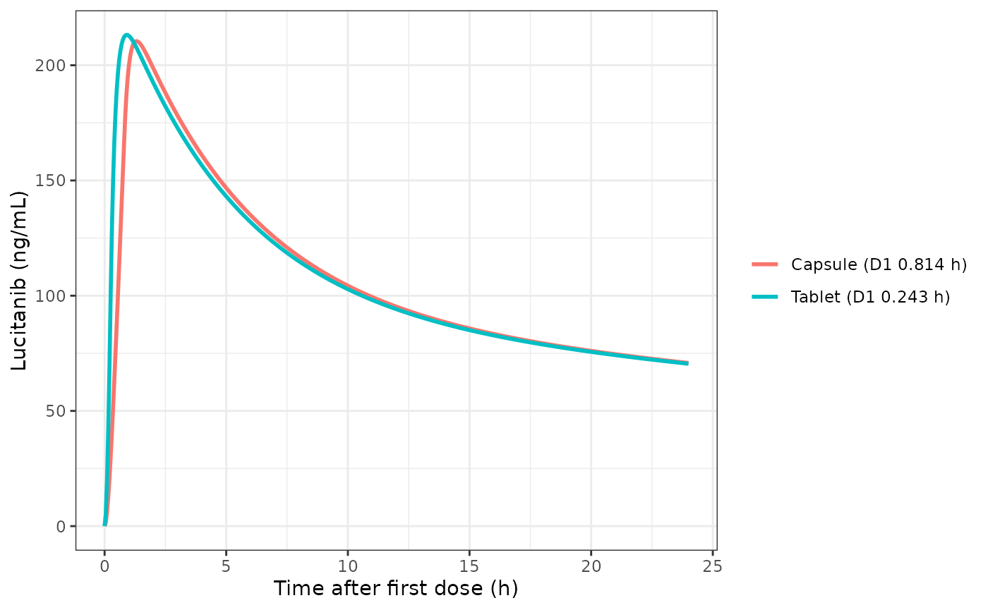
Typical-value lucitanib concentrations over the first 15 mg once-daily dosing interval, capsule versus tablet, 70 kg patient.
The checks below combine model identities (the steady-state AUC over a dosing interval must equal dose / (CL/F) regardless of the absorption shape) with statements in the text of Liao 2022.
d1_capsule <- 0.814
d1_tablet <- d1_capsule * 0.299
t_half_abs <- log(2) / 4.86
auc_closed <- 1000 * 15 / 1.90 # ng*h/mL; F = 1, CL/F = 1.90 L/h at 70 kg

k <- 1.90 / 63.8
k12 <- 6.23 / 63.8
k21 <- 6.23 / 69.1
s <- k + k12 + k21
beta <- (s - sqrt(s^2 - 4 * k * k21)) / 2
t_half_terminal <- log(2) / beta

cap <- typ[typ$FORM_TABLET == 0, ]
tab <- typ[typ$FORM_TABLET == 1, ]
r_acc <- cap$auc_ss / cap$auc_d1
t_half_eff <- 24 * log(2) / log(r_acc / (r_acc - 1))

checks <- data.frame(
  Quantity = c(
    "Tablet D1 (h)",
    "D1 reduction, tablet vs capsule (%)",
    "Absorption half-life log(2)/ka (h)",
    "AUCtau,ss capsule / (dose / CL/F)",
    "AUCtau,ss tablet / capsule",
    "Cmax day 1, tablet / capsule",
    "Cmax,ss, tablet / capsule",
    "Accumulation ratio AUCtau,ss / AUC0-24 day 1 (capsule)",
    "Effective half-life from accumulation (h)",
    "Terminal half-life log(2)/beta (h)"
  ),
  Model = vapply(signif(c(
    d1_tablet, 100 * (1 - 0.299), t_half_abs,
    cap$auc_ss / auc_closed, tab$auc_ss / cap$auc_ss,
    tab$cmax_d1 / cap$cmax_d1, tab$cmax_ss / cap$cmax_ss,
    r_acc, t_half_eff, t_half_terminal
  ), 4), format, character(1)),
  Paper = c(
    "0.243 (Abstract, Figure 1)", "70 (Discussion)", "0.143 (Discussion)",
    "--", "1 ('AUC would not be influenced', Discussion)",
    "'minimal' (Discussion)", "'minimal' (Discussion)", "--",
    "~31-40 (Discussion, citing an earlier NCA)", "--"
  )
)
knitr::kable(checks, caption = "Typical-value checks, 15 mg once daily, 70 kg patient.")| Quantity | Model | Paper |
|---|---|---|
| Tablet D1 (h) | 0.2434 | 0.243 (Abstract, Figure 1) |
| D1 reduction, tablet vs capsule (%) | 70.1 | 70 (Discussion) |
| Absorption half-life log(2)/ka (h) | 0.1426 | 0.143 (Discussion) |
| AUCtau,ss capsule / (dose / CL/F) | 1 | – |
| AUCtau,ss tablet / capsule | 1 | 1 (‘AUC would not be influenced’, Discussion) |
| Cmax day 1, tablet / capsule | 1.013 | ‘minimal’ (Discussion) |
| Cmax,ss, tablet / capsule | 1.007 | ‘minimal’ (Discussion) |
| Accumulation ratio AUCtau,ss / AUC0-24 day 1 (capsule) | 3.051 | – |
| Effective half-life from accumulation (h) | 41.9 | ~31-40 (Discussion, citing an earlier NCA) |
| Terminal half-life log(2)/beta (h) | 52.78 | – |
stopifnot(
  abs(d1_tablet - 0.243) < 5e-4,
  abs(t_half_abs - 0.143) < 5e-4,
  # Steady state reached: successive intervals agree.
  all(abs(typ$auc_ss / typ$auc_prev - 1) < 1e-3),
  # Identity: AUCtau,ss = dose / (CL/F) for both formulations (0.05 h grid).
  all(abs(typ$auc_ss / auc_closed - 1) < 1e-3),
  # The formulation changes only the release duration, so the peak moves by a
  # few percent at most; a 10-fold D1 error would move it by more than 10%.
  abs(tab$cmax_d1 / cap$cmax_d1 - 1) < 0.05,
  abs(tab$cmax_ss / cap$cmax_ss - 1) < 0.05
)
The tablet D1, the 70% shorter release and the 0.143 h absorption half-life reproduce the paper’s figures exactly, and the tablet raises the typical Cmax by about 1% with no change in AUC, the basis of the authors’ conclusion that the formulation effect is not clinically meaningful. The effective half-life from accumulation (about 42 h) sits just above the ~31-40 h the Discussion quotes from the earlier non-compartmental analysis of the first-in-human study; the model’s terminal disposition half-life is about 53 h. The paper reports no model-based half-life, so neither value is gated.
Virtual cohort
Observed data are not public. The virtual cohort reproduces the dominant regimens of the pooled data: 10 mg and 15 mg once daily as the capsule, continuously for 125 days (3000 h, the span of Figure 3). Body weight is log-normal around the Table 3 median of 67.5 kg with a 20% coefficient of variation (the paper prints no SD), redrawn when outside the Table 3 range 35.9-159 kg. Sampling follows the first-in-human schedule (Table 1): pre-dose and 1, 2, 3, 4, 6, 8, 12 and 24 h after the first dose and after the day-28 dose, plus pre-dose samples on days 4, 7, 14 and 21 and every 7 days thereafter.
set.seed(20220718)
rxode2::rxSetSeed(20220718)
n_per_arm <- 200
n_days_vpc <- 125

draw_in_range <- function(n, median, cv, lo, hi) {
  x <- stats::rlnorm(n, log(median), sqrt(log(1 + cv^2)))
  bad <- x < lo | x > hi
  while (any(bad)) {
    x[bad] <- stats::rlnorm(sum(bad), log(median), sqrt(log(1 + cv^2)))
    bad <- x < lo | x > hi
  }
  x
}

make_cohort <- function(dose, id_offset) {
  data.frame(
    id = id_offset + seq_len(n_per_arm),
    dose = dose,
    treatment = paste(dose, "mg QD"),
    WT = draw_in_range(n_per_arm, 67.5, 0.20, 35.9, 159),
    FORM_TABLET = 0
  )
}
cohort <- dplyr::bind_rows(make_cohort(10, 0L), make_cohort(15, n_per_arm))
stopifnot(!anyDuplicated(cohort$id))

rich <- c(0, 1, 2, 3, 4, 6, 8, 12, 24)
obs_times <- sort(unique(c(
  rich, 24 * 27 + rich,
  24 * c(3, 6, 13, 20), 24 * seq(34, n_days_vpc - 1, by = 7)
)))

dose_rows <- cohort |>
  dplyr::select(id, dose) |>
  tidyr::crossing(day = seq_len(n_days_vpc)) |>
  dplyr::transmute(id, time = 24 * (day - 1), amt = dose, evid = 1L, rate = -2, cmt = "depot")
obs_rows <- cohort |>
  dplyr::select(id) |>
  tidyr::crossing(time = obs_times) |>
  dplyr::mutate(amt = 0, evid = 0L, rate = 0, cmt = "central")
events <- dplyr::bind_rows(dose_rows, obs_rows) |>
  dplyr::left_join(cohort, by = "id") |>
dplyr::arrange(id, time, dplyr::desc(evid))Replicate published figures
sim |>
  dplyr::group_by(treatment, time) |>
  dplyr::summarise(
    p025 = stats::quantile(Cc, 0.025), p50 = stats::median(Cc),
    p975 = stats::quantile(Cc, 0.975), .groups = "drop"
  ) |>
  ggplot(aes(time, p50, colour = treatment, fill = treatment)) +
  geom_ribbon(aes(ymin = p025, ymax = p975), alpha = 0.2, colour = NA) +
  geom_line(linewidth = 0.8) +
  labs(
    x = "Time since first dose (h)", y = "Plasma lucitanib concentration (ng/mL)",
    colour = NULL, fill = NULL
  ) +
  theme_bw()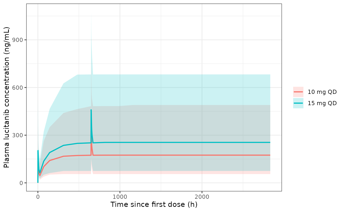
Simulated lucitanib concentrations versus time since first dose (median and 2.5th-97.5th percentiles), 10 and 15 mg once daily as the capsule. Replicates the layout of Figure 3 of Liao 2022, whose prediction intervals pool all studies, doses and sampling times.
Figure 3 of Liao 2022 shows a simulated median of roughly 150-300 ng/mL from the second week onward and a 97.5th percentile of about 1000 ng/mL, over a dataset dominated by 10 and 15 mg doses sampled at mixed times after dose. The simulated medians here (trough to peak about 170-330 ng/mL at 10 mg and 250-470 ng/mL at 15 mg on day 28; PKNCA table below) are in that range; the published figure cannot be compared point by point because it mixes doses and sampling times.
sim |>
  dplyr::distinct(id, .keep_all = TRUE) |>
  ggplot(aes(WT, cl)) +
  geom_point(alpha = 0.4) +
  geom_function(fun = function(w) 1.90 * (w / 70)^0.75, colour = "steelblue", linewidth = 1) +
  scale_y_log10() +
  labs(x = "Body weight (kg)", y = "Individual CL/F (L/h)") +
  theme_bw()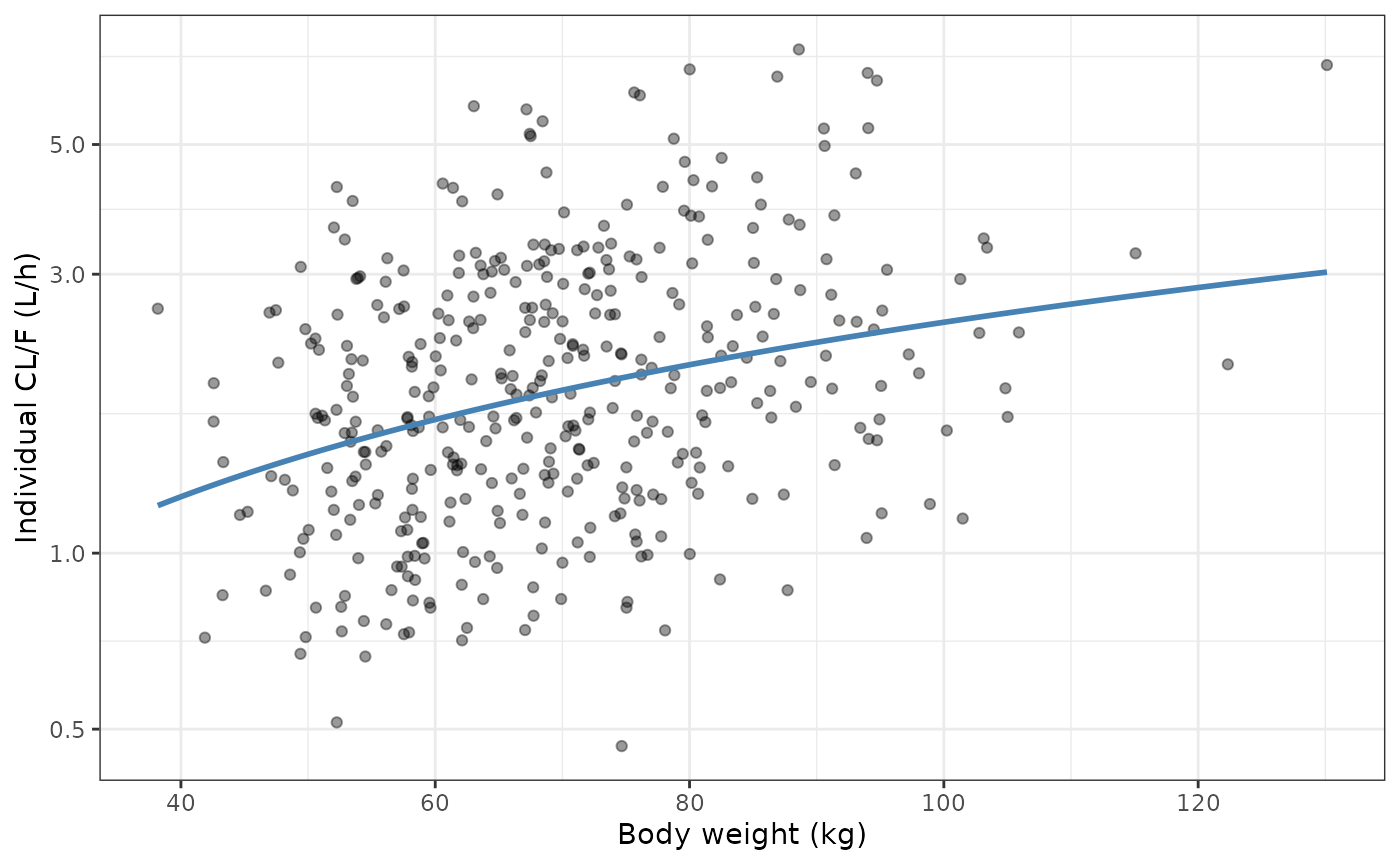
Individual CL/F versus body weight in the virtual cohort. The line is the typical-value allometric relationship 1.90 x (WT/70)^0.75.
PKNCA validation
The paper reports no NCA table, so PKNCA characterises the first dosing interval and the day-28 interval, and checks the steady-state identity AUCtau = dose / (CL/F) subject by subject with the individual CL/F from the solve.
sim_nca <- sim |>
  dplyr::filter(!is.na(Cc)) |>
  dplyr::select(id, time, Cc, treatment)

conc_obj <- PKNCA::PKNCAconc(sim_nca, Cc ~ time | treatment + id, concu = "ng/mL", timeu = "h")
dose_df <- events |>
  dplyr::filter(evid == 1) |>
  dplyr::select(id, time, amt, treatment)
dose_obj <- PKNCA::PKNCAdose(dose_df, amt ~ time | treatment + id, doseu = "mg")

intervals <- data.frame(
  start = c(0, 24 * 27), end = c(24, 24 * 28),
  cmax = TRUE, tmax = TRUE, auclast = TRUE,
  cmin = c(FALSE, TRUE), cav = c(FALSE, TRUE)
)
nca_res <- PKNCA::pk.nca(PKNCA::PKNCAdata(conc_obj, dose_obj, intervals = intervals))
nca_tab <- as.data.frame(nca_res)

nca_tab |>
  dplyr::filter(PPTESTCD %in% c("cmax", "tmax", "auclast", "cmin", "cav")) |>
  dplyr::mutate(Interval = ifelse(start == 0, "Day 1", "Day 28")) |>
  dplyr::group_by(treatment, Interval, PPTESTCD) |>
  dplyr::summarise(median = signif(stats::median(PPORRES), 3), .groups = "drop") |>
  tidyr::pivot_wider(names_from = PPTESTCD, values_from = median) |>
  dplyr::rename(
    Treatment = treatment, `Cmax (ng/mL)` = cmax, `Tmax (h)` = tmax,
    `AUCtau (ng*h/mL)` = auclast, `Cmin (ng/mL)` = cmin, `Cav (ng/mL)` = cav
  ) |>
knitr::kable(caption = "Median simulated NCA, first dose and day 28 (capsule).")| Treatment | Interval | AUCtau (ng*h/mL) | Cmax (ng/mL) | Tmax (h) | Cav (ng/mL) | Cmin (ng/mL) |
|---|---|---|---|---|---|---|
| 10 mg QD | Day 1 | 1690 | 144 | 1.5 | NA | NA |
| 10 mg QD | Day 28 | 5430 | 332 | 1.0 | 226 | 174 |
| 15 mg QD | Day 1 | 2460 | 211 | 1.5 | NA | NA |
| 15 mg QD | Day 28 | 7820 | 473 | 1.0 | 326 | 252 |
ind <- sim |>
  dplyr::distinct(id, .keep_all = TRUE) |>
  dplyr::select(id, cl, dose)
idchk <- nca_tab |>
  dplyr::filter(PPTESTCD == "auclast", start == 24 * 27) |>
  dplyr::left_join(ind, by = "id") |>
  dplyr::mutate(ratio = PPORRES / (1000 * dose / cl))
stopifnot(
  nrow(idchk) == 2 * n_per_arm,
  # A 9-point grid puts a few percent of trapezoid error on the narrow peak, and
  # subjects with a large Vp/F are not fully at steady state by day 28; a
  # transcribed CL/F, dose or unit error moves the ratio by tens of percent.
  abs(stats::median(idchk$ratio) - 1) < 0.05,
  stats::quantile(abs(idchk$ratio - 1), 0.9) < 0.15
)
The median day-28 AUCtau equals dose / (CL/F) to within a few percent, so the simulated exposure is consistent with the Table 4 clearance at both dose levels.
Assumptions and deviations
- IIV scale. Table 4 reports between-subject variability as “log-proportional, %” without saying whether the percentage is the square root of the variance or the coefficient of variation of the log-normal parameter. The maintainers converted it as a coefficient of variation, omega^2 = log(1 + CV^2), following the package convention. If the percentages are instead the square root of the variance, the variances would be 0.228 (CL/F), 0.343 (Vc/F), 0.361 (D1) and 0.588 (Vp/F); the published bootstrap percentile intervals do not distinguish the two readings.
- Residual error. The control stream codes a combined error with the additive SD fixed to 0, so the model carries the proportional term only.
-
Formulation coding. The control stream applies
THETA(10) (0.299, “tablet to capsule ratio”) as
THETA(10)**FORM, and the Abstract gives D1 = 0.243 h for the tablet, soFORM = 1is the tablet and the capsule is the reference. The formulation indicator applies per dose record. -
Covariates not retained. The P-gp-inhibitor effect
on CL/F and the albumin effect on Vc/F were added in forward selection
and removed at backward elimination; they appear in the final control
stream only as
1 FIXmultipliers and are omitted here. The formulation effect on F1 (1 FIX) is likewise omitted. Concomitant PPI on ka was statistically significant but not included in the final model (Supplemental Table 1 model 13). - Virtual cohort. Body weight is log-normal around the Table 3 median with a 20% coefficient of variation because the paper prints only the median and range. Weight is held constant per subject, although the analysis dataset coded covariates as time-varying.
- Correction notices. None found for Liao 2022 as of 2026-10-05; the only lucitanib correction notice in Europe PMC concerns the earlier first-in-human report the Discussion cites for the ~31-40 h half-life.