Piperacillin (Sanches 2022)
Source:vignettes/articles/Sanches_2022_piperacillin.Rmd
Sanches_2022_piperacillin.RmdModel and source
- Citation: Sanches C, Alves GCS, Farkas A, da Silva SD, de Castro WV, Chequer FMD, Beraldi-Magalhaes F, Magalhaes IRdS, Baldoni AdO, Chatfield MD, Lipman J, Roberts JA, Parker SL. Population Pharmacokinetic Model of Piperacillin in Critically Ill Patients and Describing Interethnic Variation Using External Validation. Antibiotics (Basel). 2022;11(4):434. doi:10.3390/antibiotics11040434
- Description: Two-compartment IV-infusion population PK model for piperacillin in critically ill Brazilian adults, with clearance proportional to Cockcroft-Gault creatinine clearance normalised to 60 mL/min/1.73 m^2 and distribution written as the central-to-peripheral and peripheral-to-central rate constants KCP and KPC. Estimated with the Pmetrics non-parametric adaptive grid (NPAG) algorithm; the NPAG marginal means are the typical values and the reported %CV values are carried as log-normal between-subject variability. The fitted model also estimated per-subject initial conditions for the day-5 sampling interval, which are not reported, so a simulation from treatment start reaches concentrations well above the paper’s observed day-5 data (see the vignette Assumptions and deviations) (Sanches 2022)
- Article: https://doi.org/10.3390/antibiotics11040434 (open access)
Population
Sanches 2022 fitted the model to 24 critically ill adults in the intensive care unit of a medium-sized hospital in Minas Gerais, Brazil, who were treated with piperacillin/tazobactam for a confirmed or suspected infection (Table 1). Median age was 72 years (IQR 57-78), median weight 69 kg (57-77), median body mass index 22 kg/m^2 (21-31), and 9 of 24 patients (38%) were male. Median Cockcroft-Gault creatinine clearance was 60 mL/min/1.73 m^2 (47-83). Half had sepsis, 29% received vasoactive drugs and 33% died; median SAPS 3 was 53, SOFA 5 and MODS 3. Patients with serum creatinine above 2 mg/dL were excluded.
Patients came from a randomised trial and received 4 g every 8 h as a roughly 30-minute infusion, or 2 g every 6 h or 3.3 g every 4 h under an individually designed dosing strategy. One or two plasma samples per patient were taken within a dosing interval on day 5 of treatment, and total piperacillin was assayed by HPLC-UV over 2.5-100 mg/L. The model was estimated in Pmetrics 1.5.0 with the non-parametric adaptive grid (NPAG) algorithm. It was then externally validated against 20 Australian and 10 Indigenous Australian ICU patients.
The same information is available programmatically via
readModelDb("Sanches_2022_piperacillin")()$population.
Source trace
| Equation / parameter | Value | Source location |
|---|---|---|
| Two-compartment model, linear elimination from central, KCP / KPC distribution | n/a | Section 2 (Results), first paragraph; section 4.3 step (i) |
CL = TVCL * (CRCL / 60) |
n/a | Section 2 (Results), first paragraph |
lcl (TVCL at CRCL 60) |
log(3.33) L/h | Table 2, CL mean (SD 1.24; median 3.01; CV 37%) |
lvc (V) |
log(10.69) L | Table 2, V mean (SD 4.50; median 9.03; CV 42%) |
lk12 (KCP) |
log(1.15) 1/h | Table 2, KCP mean (SD 0.15; median 1.21; CV 13%) |
lk21 (KPC) |
log(0.08) 1/h | Table 2, KPC mean (SD 0.09; median 0.03; CV 120%) |
etalcl, etalvc, etalk12,
etalk21
|
log(1 + CV^2) = 0.1284, 0.1625, 0.0168, 0.8920 | Table 2, %CV column |
addSd, propSd (assay SD polynomial C0,
C1) |
1 mg/L, 0.1 | Section 2: ’gamma * (1 + 0.1*concentration)’; section 4.3 step (ii) |
gammaSd |
5 | Section 2: ‘value = 5’ |
Residual: SD = gamma * (C0 + C1 * C)
|
n/a | Section 4.3 step (ii): ‘error = SD.gamma’ |
Deterministic checks of the encoding
A single 4 g dose infused over 0.5 h is solved for the typical patient at the four creatinine clearances Sanches 2022 simulated (30, 60, 90 and 130 mL/min/1.73 m^2). Two quantities are compared against closed forms built from the paper’s printed numbers, never from model output:
- AUC from zero to infinity must equal
Dose / CL, withCL = 3.33 * CRCL / 60. - The terminal half-life must equal
log(2) / beta, the slower root ofx^2 - (kel + KCP + KPC) x + kel * KPC = 0. A two-compartment model whose peripheral compartment had been dropped would instead decay atkel, and the AUC check alone would not notice.
mod <- readModelDb("Sanches_2022_piperacillin")
mod_typical <- rxode2::zeroRe(mod)
#> ℹ parameter labels from comments will be replaced by 'label()'
#> Warning: No sigma parameters in the model

crcl_levels <- c(30, 60, 90, 130)
obs_times <- sort(unique(c(
  0,
  seq(0.05, 2, by = 0.05),
  seq(2.5, 48, by = 0.5),
  seq(50, 1500, by = 5)
)))

ev_sd <- bind_rows(lapply(seq_along(crcl_levels), function(i) {
  bind_rows(
    tibble(id = i, time = 0, evid = 1, amt = 4000, rate = 8000, cmt = "central"),
    tibble(id = i, time = obs_times, evid = 0, amt = 0, rate = 0, cmt = "central")
  ) |>
    mutate(CRCL = crcl_levels[i], treatment = paste0("CRCL ", crcl_levels[i]))
})) |>
  arrange(id, time, desc(evid))

sim_sd <- rxode2::rxSolve(
  mod_typical,
  events = ev_sd,
  keep = c("CRCL", "treatment"),
  rtol = 1e-10,
  atol = 1e-12,
  maxsteps = 1e6
) |>
  as.data.frame()
#> ℹ omega/sigma items treated as zero: 'etalcl', 'etalvc', 'etalk12', 'etalk21'
#> Warning: multi-subject simulation without without 'omega'

# The peripheral compartment must survive the solve.
stopifnot("peripheral1" %in% names(sim_sd))
stopifnot(all(sim_sd$Cc >= -1e-6 * max(sim_sd$Cc)))
beta_root <- function(crcl) {
  kel <- 3.33 * crcl / 60 / 10.69
  a <- kel + 1.15 + 0.08
  b <- kel * 0.08
  (a - sqrt(a^2 - 4 * b)) / 2
}

# Log-linear slope over 100-300 h, long after the distribution phase
# (alpha > 1.3 1/h at every CRCL) has died out.
hl_check <- sim_sd |>
  filter(time >= 100, time <= 300) |>
  group_by(treatment, CRCL) |>
  summarise(slope = -coef(lm(log(Cc) ~ time))[2], .groups = "drop") |>
  mutate(
    hl_sim = log(2) / slope,
    hl_closed = log(2) / beta_root(CRCL),
    hl_kel = log(2) / (3.33 * CRCL / 60 / 10.69),
    ratio = hl_sim / hl_closed
  )

hl_check |>
  select(treatment, hl_sim, hl_closed, hl_kel, ratio) |>
  rename(
    "Group" = treatment,
    "Simulated terminal t1/2 (h)" = hl_sim,
    "Closed-form log(2)/beta (h)" = hl_closed,
    "log(2)/kel, if the peripheral were lost (h)" = hl_kel,
    "Ratio" = ratio
  ) |>
knitr::kable(digits = 3, caption = "Terminal half-life, typical patient.")| Group | Simulated terminal t1/2 (h) | Closed-form log(2)/beta (h) | log(2)/kel, if the peripheral were lost (h) | Ratio |
|---|---|---|---|---|
| CRCL 130 | 24.085 | 24.085 | 1.027 | 1 |
| CRCL 30 | 76.584 | 76.584 | 4.450 | 1 |
| CRCL 60 | 42.422 | 42.422 | 2.225 | 1 |
| CRCL 90 | 31.058 | 31.058 | 1.483 | 1 |
# Deterministic: same parameters on both sides, so only integrator error.
stopifnot(all(abs(hl_check$ratio - 1) < 1e-4))
The terminal half-life is long: about 42 h at a creatinine clearance
of 60 mL/min/1.73 m^2 and 77 h at 30. This follows from the published
KPC of 0.08 1/h, which gives a peripheral volume of
V * KCP / KPC, about 154 L, and a steady-state volume near
165 L.
PKNCA validation
conc_df <- sim_sd |>
  filter(!is.na(Cc)) |>
  mutate(Cc = pmax(Cc, 0)) |>
  select(id, time, Cc, treatment)

dose_df <- ev_sd |>
  filter(evid == 1) |>
  select(id, time, amt, treatment)

conc_obj <- PKNCA::PKNCAconc(conc_df, Cc ~ time | treatment + id)
dose_obj <- PKNCA::PKNCAdose(dose_df, amt ~ time | treatment + id, route = "intravascular", duration = 0.5)

intervals <- data.frame(
  start = 0,
  end = Inf,
  cmax = TRUE,
  tmax = TRUE,
  aucinf.obs = TRUE,
  half.life = TRUE
)

nca_res <- PKNCA::pk.nca(PKNCA::PKNCAdata(conc_obj, dose_obj, intervals = intervals))

nca_tab <- as.data.frame(nca_res$result) |>
  filter(PPTESTCD %in% c("cmax", "tmax", "aucinf.obs", "half.life")) |>
  select(treatment, PPTESTCD, PPORRES) |>
  pivot_wider(names_from = PPTESTCD, values_from = PPORRES) |>
  mutate(
    CRCL = as.numeric(sub("CRCL ", "", treatment)),
    auc_closed = 4000 / (3.33 * CRCL / 60),
    auc_ratio = aucinf.obs / auc_closed
  )

nca_tab |>
  select(treatment, cmax, tmax, aucinf.obs, auc_closed, auc_ratio, half.life) |>
  rename(
    "Group" = treatment,
    "Cmax (mg/L)" = cmax,
    "Tmax (h)" = tmax,
    "AUC0-inf (mg*h/L)" = aucinf.obs,
    "Dose/CL (mg*h/L)" = auc_closed,
    "AUC ratio" = auc_ratio,
    "t1/2 (h)" = half.life
  ) |>
knitr::kable(digits = 3, caption = "PKNCA, single 4 g dose over 0.5 h, typical patient.")| Group | Cmax (mg/L) | Tmax (h) | AUC0-inf (mg*h/L) | Dose/CL (mg*h/L) | AUC ratio | t1/2 (h) |
|---|---|---|---|---|---|---|
| CRCL 130 | 246.337 | 0.5 | 554.649 | 554.401 | 1 | 24.062 |
| CRCL 30 | 275.824 | 0.5 | 2402.876 | 2402.402 | 1 | 76.507 |
| CRCL 60 | 266.473 | 0.5 | 1201.597 | 1201.201 | 1 | 42.368 |
| CRCL 90 | 257.565 | 0.5 | 801.128 | 800.801 | 1 | 31.013 |
# AUC0-inf = Dose/CL for any linear model; the trapezoid on this grid is well
# inside 1%.
stopifnot(all(abs(nca_tab$auc_ratio - 1) < 0.01))
Sanches 2022 reports no NCA parameters, so there is no published NCA table to compare against.
Day-5 concentrations against the observed data
Figure 1C of Sanches 2022 is a VPC of the day-5 sampling interval. It shows a peak cloud up to about 95 mg/L in the first two hours after the start of the infusion and a trough plateau of roughly 5-30 mg/L. No observed concentration exceeded 100 mg/L (Discussion, limitation (d)). The chunk below simulates 200 virtual patients on 4 g every 8 h from the first dose to the day-5 interval (96-104 h). Their creatinine clearances are drawn from a log-normal with the Table 1 median of 60 mL/min/1.73 m^2 and an IQR near 47-83.
rxode2::rxSetSeed(20220324)
n_vpc <- 200
crcl_vpc <- exp(rnorm(n_vpc, log(60), log(83 / 47) / 1.349))

dose_times_q8 <- seq(0, 96, by = 8)
vpc_times <- seq(96, 104, by = 0.1)

ev_vpc <- bind_rows(lapply(seq_len(n_vpc), function(i) {
  bind_rows(
    tibble(id = i, time = dose_times_q8, evid = 1, amt = 4000, rate = 8000, cmt = "central"),
    tibble(id = i, time = vpc_times, evid = 0, amt = 0, rate = 0, cmt = "central")
  ) |>
    mutate(CRCL = crcl_vpc[i])
})) |>
  arrange(id, time, desc(evid))

sim_vpc <- rxode2::rxSolve(mod, events = ev_vpc, keep = "CRCL", maxsteps = 1e6) |>
  as.data.frame() |>
  mutate(tad = time - 96)
#> ℹ parameter labels from comments will be replaced by 'label()'

vpc_sum <- sim_vpc |>
  group_by(tad) |>
  summarise(
    Q05 = quantile(Cc, 0.05),
    Q50 = quantile(Cc, 0.50),
    Q95 = quantile(Cc, 0.95),
    .groups = "drop"
  )

ggplot(vpc_sum, aes(tad, Q50)) +
  geom_ribbon(aes(ymin = Q05, ymax = Q95), alpha = 0.25) +
  geom_line() +
  geom_hline(yintercept = 100, linetype = "dashed") +
  annotate("text", x = 6, y = 108, label = "highest observed concentration < 100 mg/L") +
  labs(
    x = "Time after the day-5 dose (h)",
    y = "Total piperacillin Cc (mg/L)",
    title = "Day-5 interval, 4 g every 8 h from treatment start",
    caption = "Compare with Figure 1C of Sanches 2022 (observed day-5 data 5-95 mg/L)."
  )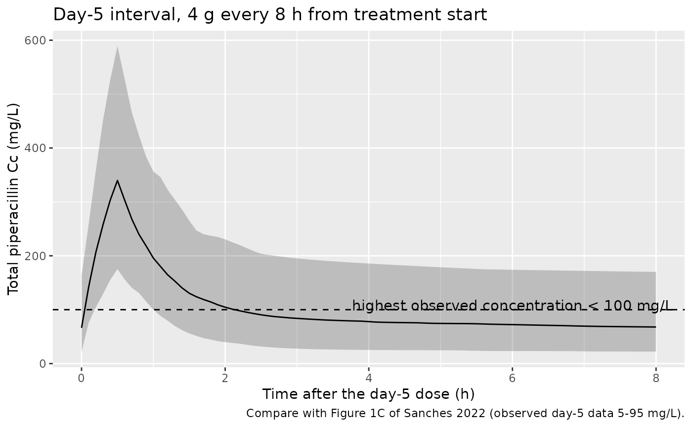
The simulated median trough at the end of the day-5 interval is 67.9 mg/L. 45% of simulated day-5 concentrations exceed 100 mg/L. Both are well above the observed data in Figure 1C. The cause is described in Assumptions and deviations: the fitted model estimated each patient’s day-5 starting amounts as initial conditions rather than simulating the preceding four days of dosing, and those estimates are not published.
Replicate Figure 2 (probability of target attainment)
Sanches 2022 Figure 2 gives the probability that free piperacillin, with 30% protein binding, exceeds each MIC for at least 50% or 100% of a dosing interval. It covers 4 g every 8 h (A) and every 6 h (B), each as a 0.5 h infusion, at creatinine clearances of 30, 60, 90 and 130 mL/min/1.73 m^2. The Results describe Figure 2 as the fifth day of treatment and section 4.5 as a steady-state interval. The simulation below uses the day-5 interval from treatment start, 200 virtual patients per regimen and creatinine clearance, without residual error.
rxode2::rxSetSeed(20220325)
n_arm <- 200
fu <- 0.7
mics <- 2^(-3:7)

make_pta_arm <- function(tau, crcl, id_offset) {
  dose_times <- seq(0, 96, by = tau)
  obs <- seq(96, 96 + tau, by = 0.05)
  bind_rows(lapply(seq_len(n_arm), function(i) {
    bind_rows(
      tibble(id = id_offset + i, time = dose_times, evid = 1, amt = 4000, rate = 8000, cmt = "central"),
      tibble(id = id_offset + i, time = obs, evid = 0, amt = 0, rate = 0, cmt = "central")
    )
  })) |>
    mutate(CRCL = crcl, tau = tau, regimen = paste0("4 g q", tau, "h"))
}

arms <- expand.grid(tau = c(8, 6), crcl = crcl_levels)
ev_pta <- bind_rows(lapply(seq_len(nrow(arms)), function(k) {
  make_pta_arm(arms$tau[k], arms$crcl[k], id_offset = (k - 1L) * n_arm)
})) |>
  arrange(id, time, desc(evid))
stopifnot(!anyDuplicated(ev_pta[ev_pta$evid == 1, c("id", "time")]))

sim_pta <- rxode2::rxSolve(mod, events = ev_pta, keep = c("CRCL", "tau", "regimen"), maxsteps = 1e6) |>
  as.data.frame() |>
  filter(time >= 96)

# Fraction of the interval with free concentration above the MIC, by the
# rectangle rule on the 0.05 h grid (last grid point excluded).
ft_by_id <- sim_pta |>
  group_by(id, regimen, CRCL, tau) |>
  filter(time < 96 + first(tau)) |>
  reframe(MIC = mics, ft = sapply(mics, function(m) mean(fu * Cc > m)))

pta <- ft_by_id |>
  group_by(regimen, CRCL, MIC) |>
  summarise(
    `50% fT>MIC` = 100 * mean(ft >= 0.5),
    `100% fT>MIC` = 100 * mean(ft >= 1),
    .groups = "drop"
  ) |>
  pivot_longer(c(`50% fT>MIC`, `100% fT>MIC`), names_to = "target", values_to = "PTA")
ggplot(pta, aes(MIC, PTA, colour = factor(CRCL))) +
  geom_line() +
  geom_point() +
  geom_hline(yintercept = 90, linetype = "dashed") +
  scale_x_log10(breaks = mics, labels = as.character(mics)) +
  facet_grid(target ~ regimen) +
  labs(
    x = "MIC (mg/L)", y = "PTA (%)", colour = "CRCL\n(mL/min/1.73 m^2)",
    caption = "Replicates Figure 2 of Sanches 2022 (day-5 interval; fu = 0.7)."
  )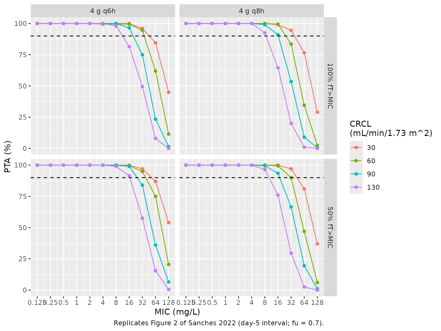
The Figure 2 points were digitised by the maintainers. Panel A1 was read from a 250 dpi render (about +/- 1 PTA point); the other panels at MIC 8 and 16 were read from a 110 dpi render (about +/- 2 points).
published <- tribble(
  ~regimen, ~target, ~MIC, ~CRCL, ~PTA_pub,
  "4 g q8h", "50% fT>MIC", 8, 30, 99,
  "4 g q8h", "50% fT>MIC", 8, 60, 94,
  "4 g q8h", "50% fT>MIC", 8, 90, 87,
  "4 g q8h", "50% fT>MIC", 8, 130, 74,
  "4 g q8h", "50% fT>MIC", 16, 30, 82,
  "4 g q8h", "50% fT>MIC", 16, 60, 59,
  "4 g q8h", "50% fT>MIC", 16, 90, 36,
  "4 g q8h", "50% fT>MIC", 16, 130, 14,
  "4 g q8h", "100% fT>MIC", 8, 30, 92,
  "4 g q8h", "100% fT>MIC", 8, 60, 87,
  "4 g q8h", "100% fT>MIC", 8, 90, 80,
  "4 g q8h", "100% fT>MIC", 8, 130, 61,
  "4 g q8h", "100% fT>MIC", 16, 30, 68,
  "4 g q8h", "100% fT>MIC", 16, 60, 43,
  "4 g q8h", "100% fT>MIC", 16, 90, 20,
  "4 g q8h", "100% fT>MIC", 16, 130, 5,
  "4 g q6h", "50% fT>MIC", 16, 30, 82,
  "4 g q6h", "50% fT>MIC", 16, 60, 63,
  "4 g q6h", "50% fT>MIC", 16, 90, 38,
  "4 g q6h", "50% fT>MIC", 16, 130, 15,
  "4 g q6h", "100% fT>MIC", 16, 30, 69,
  "4 g q6h", "100% fT>MIC", 16, 60, 45,
  "4 g q6h", "100% fT>MIC", 16, 90, 20,
  "4 g q6h", "100% fT>MIC", 16, 130, 5
)

cmp <- published |>
  inner_join(pta, by = c("regimen", "target", "MIC", "CRCL")) |>
  mutate(diff = PTA - PTA_pub)
stopifnot(nrow(cmp) == nrow(published))

cmp |>
  rename(
    "Regimen" = regimen,
    "Target" = target,
    "MIC (mg/L)" = MIC,
    "CRCL" = CRCL,
    "Published PTA (%)" = PTA_pub,
    "Simulated PTA (%)" = PTA,
    "Difference (points)" = diff
  ) |>
knitr::kable(digits = 1, caption = "Figure 2 PTA: digitised published vs simulated.")| Regimen | Target | MIC (mg/L) | CRCL | Published PTA (%) | Simulated PTA (%) | Difference (points) |
|---|---|---|---|---|---|---|
| 4 g q8h | 50% fT>MIC | 8 | 30 | 99 | 100.0 | 1.0 |
| 4 g q8h | 50% fT>MIC | 8 | 60 | 94 | 100.0 | 6.0 |
| 4 g q8h | 50% fT>MIC | 8 | 90 | 87 | 99.5 | 12.5 |
| 4 g q8h | 50% fT>MIC | 8 | 130 | 74 | 96.5 | 22.5 |
| 4 g q8h | 50% fT>MIC | 16 | 30 | 82 | 100.0 | 18.0 |
| 4 g q8h | 50% fT>MIC | 16 | 60 | 59 | 99.5 | 40.5 |
| 4 g q8h | 50% fT>MIC | 16 | 90 | 36 | 93.5 | 57.5 |
| 4 g q8h | 50% fT>MIC | 16 | 130 | 14 | 76.0 | 62.0 |
| 4 g q8h | 100% fT>MIC | 8 | 30 | 92 | 100.0 | 8.0 |
| 4 g q8h | 100% fT>MIC | 8 | 60 | 87 | 100.0 | 13.0 |
| 4 g q8h | 100% fT>MIC | 8 | 90 | 80 | 99.0 | 19.0 |
| 4 g q8h | 100% fT>MIC | 8 | 130 | 61 | 92.5 | 31.5 |
| 4 g q8h | 100% fT>MIC | 16 | 30 | 68 | 99.0 | 31.0 |
| 4 g q8h | 100% fT>MIC | 16 | 60 | 43 | 99.5 | 56.5 |
| 4 g q8h | 100% fT>MIC | 16 | 90 | 20 | 91.0 | 71.0 |
| 4 g q8h | 100% fT>MIC | 16 | 130 | 5 | 64.5 | 59.5 |
| 4 g q6h | 50% fT>MIC | 16 | 30 | 82 | 100.0 | 18.0 |
| 4 g q6h | 50% fT>MIC | 16 | 60 | 63 | 99.5 | 36.5 |
| 4 g q6h | 50% fT>MIC | 16 | 90 | 38 | 99.0 | 61.0 |
| 4 g q6h | 50% fT>MIC | 16 | 130 | 15 | 91.5 | 76.5 |
| 4 g q6h | 100% fT>MIC | 16 | 30 | 69 | 100.0 | 31.0 |
| 4 g q6h | 100% fT>MIC | 16 | 60 | 45 | 99.5 | 54.5 |
| 4 g q6h | 100% fT>MIC | 16 | 90 | 20 | 96.5 | 76.5 |
| 4 g q6h | 100% fT>MIC | 16 | 130 | 5 | 81.5 | 76.5 |
The simulated PTA is systematically higher than Figure 2 at the MICs where the curves fall: median difference 34 points. This is a known deviation and is not gated. The published curves also show almost no difference between 4 g every 6 h and 4 g every 8 h, although the 6-hourly regimen delivers a third more drug per day. That is not reproducible from the Table 2 point estimates under any simulation start the maintainers tried: day 5 from treatment start, full steady state, with or without assay noise added, and with either the mean or the median column.
The one property of Figure 2 that the published model must reproduce is the direction of the creatinine-clearance effect. Clearance at 130 mL/min/1.73 m^2 is 4.3 times that at 30, so attainment at MIC 16 must fall steeply across the range:
pta_at <- function(reg, tgt, mic, crcl) {
  v <- pta$PTA[pta$regimen == reg & pta$target == tgt & pta$MIC == mic & pta$CRCL == crcl]
  if (length(v) != 1L) stop("no unique PTA row for ", reg, " / ", tgt, " / ", mic, " / ", crcl)
  v
}
drop_q8 <- pta_at("4 g q8h", "100% fT>MIC", 16, 30) - pta_at("4 g q8h", "100% fT>MIC", 16, 130)
drop_q8
#> [1] 34.5
# A 200-subject arm has a binomial SE below 3.6 points. In the Monte Carlo
# explorations the drop was about 25 points (99 -> 73) at 1000 subjects per
# arm, so 10 points is more than 3 SE clear of the model-true value. A
# clearance that ignored CRCL would give a drop near zero.
stopifnot(drop_q8 > 10)
Assumptions and deviations
- Typical values are the NPAG means. Table 2 prints mean (SD), median and %CV for each parameter. The Abstract and Results quote the means, and the %CV column is SD/mean (1.24/3.33 = 37%, 4.50/10.69 = 42%, 0.15/1.15 = 13%), so the means are encoded. For KPC the rounded values give 0.09/0.08 = 113% against the printed 120%; the printed %CV is used. The medians (CL 3.01 L/h, V 9.03 L, KCP 1.21 1/h, KPC 0.03 1/h) are lower. For KPC the median is less than half the mean, a sign that the non-parametric marginal is far from log-normal. Re-simulating the paper’s own Figure 2 did not favour either column; both gave attainment well above the published curves.
-
Between-subject variability is a log-normal
approximation. NPAG estimates a discrete joint density over
support points, not an omega matrix. Each marginal is represented by a
log-normal with the printed %CV,
omega^2 = log(1 + CV^2). No correlations are published, so the etas are independent. Any multimodality in the NPAG density cannot be recovered. -
Initial conditions are not reproduced. Section 2
states that the final model included ‘initial conditions to describe the
steady-state conditions achieved prior to the dosing interval’. Each
patient’s starting amounts at the sampled day-5 interval were therefore
estimated, rather than generated by simulating the preceding days of
dosing, and the estimates are not published. The model here starts empty
at the first dose. Combined with the long terminal half-life implied by
KPC = 0.08 1/h (about 42 h at CRCL 60), this means a simulation from
treatment start accumulates to day-5 concentrations well above the
observed data. At true steady state the average total concentration of 4
g every 8 h is
Dose / (tau * CL), about 150 mg/L at CRCL 60, whereas no observed concentration exceeded 100 mg/L. The model was fitted to a single dosing interval per patient, so its multiple-dose predictions should be used with that caution. - Figure 2 is not reproduced. See the PTA section: the simulated attainment exceeds the published curves, and the published near-equality of the 6- and 8-hourly regimens cannot be reproduced from the published parameters. Section 4.5 says the Monte Carlo used ‘different dosing regimens, BMI and a range of creatinine clearances’. No BMI effect is in the final model, and the simulation settings beyond those stated (initial conditions, noise, sampling grid) are not published. Table 3’s fractional target attainment was not re-simulated because it also requires the EUCAST MIC distribution for P. aeruginosa, which is not given in the paper.
-
Residual error. Pmetrics weights each observation
by
SD * gammawithSD = C0 + C1 * Y, a linear sum. Here that is5 * (1 + 0.1 * Y)mg/L, encoded asadd(sdCc)withsdCc = gammaSd * (addSd + propSd * Cc). Pmetrics evaluates the polynomial on the observed concentration, whereas nlmixr2 evaluates it on the prediction. The PTA simulations above exclude residual error. -
Distribution is parameterised by rate constants.
The paper estimates KCP and KPC directly. The model derives
q = KCP * Vandvp = q / KPCand drives the ODEs through them, which is algebraically identical; the terminal half-life check above confirms the peripheral compartment is retained. - Protein binding. The 30% plasma protein binding used for the free concentrations is the paper’s assumption (section 4.5 and Discussion). It is not part of the model, which predicts total concentration.
-
Screened covariates. Age, height, weight, sex, BMI,
serum creatinine, sepsis, CKD-EPI eGFR, SAPS 3, MODS and SOFA were
screened and not retained (section 4.3 step iii). Those with a canonical
column name are documented in the model’s
covariatesDataExcluded. - Virtual cohort. Creatinine clearance in the day-5 VPC is drawn from a log-normal matched to the Table 1 median and IQR; the paper gives no distribution. The PTA arms use the paper’s fixed creatinine clearance values.
- No erratum or correction notice for Sanches 2022 is linked to the article in Europe PMC as of 2026-09-30.