Aripiprazole once monthly exposure-response in bipolar I disorder (Wang 2025)
Source:vignettes/articles/Wang_2025_aripiprazole_bipolar.Rmd
Wang_2025_aripiprazole_bipolar.RmdModels and source
Wang 2025 links aripiprazole exposure to the time to recurrence of any mood episode in adults with bipolar I disorder maintained on aripiprazole once monthly (AOM). The analysis has two layers:
-
Exposure. The previously published population PK
model of Wang 2022 was applied, with every parameter fixed, to the
bipolar trial. It is already in the library as
modellib("Wang_2022_aripiprazole"), and the supplement’s Table S2 reproduces it verbatim, so this paper adds no PK parameters. - Exposure-response. Two Cox proportional-hazards models were fitted separately to the same 265 patients: the final model, with the predicted concentration as a continuous linear predictor, and a categorical model that tests the 95 ng/mL threshold established in schizophrenia. They are packaged as two files:
-
Wang_2025_aripiprazole_recurrence(continuous, final): Cox proportional-hazards exposure-response model for the time to recurrence of any mood episode in adults with bipolar I disorder maintained on aripiprazole once monthly (AOM) 400 mg or withdrawn to placebo in the randomised double-blind withdrawal phase of trial NCT01567527 (Wang 2025, final model). The exposure driver is CTROUGH, the model-predicted aripiprazole plasma concentration 672 h (28 days) after the first injection of the double-blind phase (‘Ctau’), generated from the companion population PK model modellib(‘Wang_2022_aripiprazole’); for placebo subjects it is the residual concentration still washing out from the last open-label AOM dose. CTROUGH enters the log hazard linearly and uncentred: each 1 ng/mL increase multiplies the hazard of recurrence by exp(-0.00346) = 0.99655, a 0.34 percent reduction. No other covariate was retained. Because the fit is a semiparametric Cox regression, the baseline hazard is unspecified by construction and is not reported; the model therefore returns the RELATIVE hazard hr against a hypothetical subject with CTROUGH = 0, not an absolute survivor function. Multiply hr by a user-supplied baseline hazard h0(t) to obtain a subject hazard. The model is algebraic and deterministic (no ODE state, no drug input, no IIV, no residual error). The separately fitted categorical model that dichotomises CTROUGH at 95 ng/mL is modellib(‘Wang_2025_aripiprazole_recurrence_cutoff’). -
Wang_2025_aripiprazole_recurrence_cutoff(categorical): Cox proportional-hazards exposure-response model for the time to recurrence of any mood episode in adults with bipolar I disorder maintained on aripiprazole once monthly (AOM) 400 mg or withdrawn to placebo in the randomised double-blind withdrawal phase of trial NCT01567527 (Wang 2025, categorical model). This is the separately fitted model in which the exposure driver CTROUGH – the model-predicted aripiprazole plasma concentration 672 h after the first double-blind injection (‘Ctau’), from the companion population PK model modellib(‘Wang_2022_aripiprazole’) – enters only through the 95 ng/mL efficacy threshold previously established in schizophrenia: subjects at or above the threshold have a hazard of recurrence 0.6450-fold that of subjects below it (a 36 percent, or 1.55-fold, reduction). The authors’ preferred final model is the continuous one, modellib(‘Wang_2025_aripiprazole_recurrence’); this categorical model was fitted to allow direct comparison with the schizophrenia threshold model modellib(‘Wang_2022_aripiprazole_relapse’). Because the fit is a semiparametric Cox regression, the baseline hazard is unspecified by construction and is not reported; the model therefore returns the RELATIVE hazard hr against the below-threshold reference group, not an absolute survivor function. The model is algebraic and deterministic (no ODE state, no drug input, no IIV, no residual error). - Citation: Wang X, Phillips L, Harlin M, Bell Lynum KS, Larsen F, Such P, Madera-McDonough J, Yildirim M, Procyshyn RM, Chepke C, Passarell J. Exposure-Response Analysis for Aripiprazole Once-Monthly in Patients Diagnosed With Bipolar I Disorder. Clin Pharmacol Drug Dev. 2025;14(11):869-878. doi:10.1002/cpdd.1580. The coefficient is from the Results section ‘Exposure-Response Model’; the model equation is in Appendix S4 of the Supporting Information. The upstream population PK model that generates the CTROUGH covariate (reproduced as Appendix S2 Table S2) is Wang X, Raoufinia A, Bihorel S, et al. Clin Pharmacol Drug Dev. 2022;11(2):150-164, doi:10.1002/cpdd.1022; see modellib(‘Wang_2022_aripiprazole’).
- Article: https://doi.org/10.1002/cpdd.1580
The sibling schizophrenia analysis from the same group is
modellib("Wang_2022_aripiprazole_relapse"). There the
exposure-response model was an exponential (constant-hazard) model with
the 95 ng/mL threshold, and the hazard ratio was 1/4.41.
Population
Data come from the phase 3 trial NCT01567527 of AOM 400 mg as maintenance treatment in bipolar I disorder (Wang 2025 Methods; Appendix S1). Patients entered in a manic episode (YMRS >= 20). They were converted to oral aripiprazole and stabilised on it (Phases A and B), then stabilised on open-label AOM 400 mg every 4 weeks, with oral aripiprazole 10 or 15 mg/day for the first 14 days (Phase C, 12-28 weeks). Finally they were randomised 1:1 to continue AOM or switch to placebo injections for 52 weeks (Phase D). A single decrease to AOM 300 mg was allowed for tolerability, and 68 patients (16.2%) used it.
The exposure-response set is the 265 patients of Phase D: 132 on AOM and 133 on placebo (Table S5). Their mean (SD) age was 40.1 (11.0) years and their body mass index 30.2 (7.2) kg/m^2. 57.4% were female. By race, 54.3% were White, 27.9% Black or African American and 14.0% Asian. Mean MADRS and YMRS totals at randomisation were 2.7 and 2.8. The population PK validation set was larger, at 420 patients (Table S3). In that set, 2.9% were CYP2D6 poor metabolisers and 6.4% had an inconclusive or missing genotype. There were 103 recurrences: 35 (26.5%) on AOM and 68 (51.1%) on placebo (Table 1).
The exposure metric, Ctau in the paper and
CTROUGH here, is the model-predicted aripiprazole plasma
concentration 672 h (28 days) after the first Phase D injection. Placebo
patients received no active drug at that injection, but they were still
washing out their last open-label AOM dose, given about 1344 h (56 days)
before the landmark. So their CTROUGH is substantial and
not zero.
Source trace
| Model element | Value | Source location |
|---|---|---|
Continuous model equation
S(t) = S0(t)^exp(beta * Ctau)
|
– | Appendix S4, step 5 |
e_ctrough_haz |
-0.00346 (RSE 44%) | Results, “Exposure-Response Model” (HR 0.99655, 95% CI 0.9936-0.9995, P = .0230) |
| Linear rather than log-linear Ctau | – | Results (linear P = .0170 in univariate testing) |
| No retained covariates (age, BMI, MADRS, YMRS, sex, race screened) | – | Results; Appendix S4, step 3 |
ctrough_cut |
95 ng/mL (fixed) | Results, “Exposure-Response Model” (tested, not estimated) |
e_ctrough_cut_haz |
log(0.6450) | Results, “Exposure-Response Model” (HR 0.6450, 95% CI 0.4372-0.9514, P = .0270) |
| Ctau definition (672 h after the first Phase D dose) | – | Methods, “Development of the Exposure-Response Model” |
| Upstream PK model | Wang_2022_aripiprazole |
Methods; Appendix S2, Table S2 |
| Ctau mean (SD) by arm | AOM 170.5 (71.6); placebo 78.7 (36.1) ng/mL | Results text; Table 1 |
| Ctau quartile edges, pooled | 9.48 / 70.39 / 110.21 / 164.2 / 390.86 ng/mL | Figure 2 legend |
| N below / at or above 95 ng/mL | 111 / 154 | Figure 3 panel labels |
Model structure
Both models return the relative hazard hr = exp(lhr). In
the continuous model the reference is a hypothetical patient with
CTROUGH = 0. In the categorical model it is the group below
95 ng/mL. A Cox regression leaves the baseline hazard h0(t)
unspecified, and the paper reports no estimate of it. So neither file
offers a survivor function. To get a patient’s hazard, multiply
hr by a baseline the user supplies.
Validation
A. The published hazard ratios are reproduced exactly
Both models are deterministic and algebraic, so their output can be checked against the printed numbers to the printed precision.
# One observation row per grid point on a single subject, with the covariate
# as an event-table column. A params data.frame would be read as one row per
# subject and fail on a one-subject event table.
erEval <- function(model, grid) {
  ev <- data.frame(id = 1L, time = seq_along(grid), amt = 0, evid = 0L,
                   CTROUGH = grid)
  s <- as.data.frame(rxode2::rxSolve(model, events = ev,
                                     returnType = "data.frame"))
  stopifnot(nrow(s) == length(grid))
  s$hr
}

modCont <- readModelDb("Wang_2025_aripiprazole_recurrence")
modCut  <- readModelDb("Wang_2025_aripiprazole_recurrence_cutoff")

hrPer1 <- erEval(modCont, c(0, 1))
hrCut  <- erEval(modCut, c(0, 94.99, 95, 400))

# Continuous model: per-1 ng/mL hazard ratio is printed as 0.99655, and the
# derived per-1 ng/mL reduction as 0.34%.
coefCont <- -0.00346
seCont   <- 0.44 * abs(coefCont)   # RSE 44%
ciCont   <- exp(coefCont + c(-1, 1) * qnorm(0.975) * seCont)

hrTable <- tibble::tibble(
  quantity = c("HR per 1 ng/mL Ctau", "Hazard reduction per 1 ng/mL (%)",
               "95% CI lower (from RSE)", "95% CI upper (from RSE)",
               "HR, Ctau >= 95 vs < 95 ng/mL", "Fold reduction, 1/HR",
               "Risk reduction, 1 - HR (%)"),
  model = c(hrPer1[2] / hrPer1[1], 100 * (1 - hrPer1[2] / hrPer1[1]),
            ciCont[1], ciCont[2],
            hrCut[3] / hrCut[2], hrCut[2] / hrCut[3],
            100 * (1 - hrCut[3] / hrCut[2])),
  published = c(0.99655, 0.34, 0.9936, 0.9995, 0.6450, 1.55, 36)
)
hrTable |>
  dplyr::mutate(model = signif(model, 5)) |>
  dplyr::rename("Quantity" = quantity, "Packaged model" = model,
                "Wang 2025" = published) |>
knitr::kable()| Quantity | Packaged model | Wang 2025 |
|---|---|---|
| HR per 1 ng/mL Ctau | 0.99655 | 0.99655 |
| Hazard reduction per 1 ng/mL (%) | 0.34540 | 0.34000 |
| 95% CI lower (from RSE) | 0.99358 | 0.99360 |
| 95% CI upper (from RSE) | 0.99952 | 0.99950 |
| HR, Ctau >= 95 vs < 95 ng/mL | 0.64500 | 0.64500 |
| Fold reduction, 1/HR | 1.55040 | 1.55000 |
| Risk reduction, 1 - HR (%) | 35.50000 | 36.00000 |
stopifnot(
  # Exact reproduction, rounded to the printed precision.
  round(hrPer1[2] / hrPer1[1], 5) == 0.99655,
  # 0.345% printed as 0.34%: truncated, not rounded, hence the 0.01 window.
  abs(100 * (1 - hrPer1[2] / hrPer1[1]) - 0.34) < 0.01,
  all(abs(ciCont - c(0.9936, 0.9995)) < 1e-4),
  abs(hrCut[3] / hrCut[2] - 0.6450) < 1e-10,
  round(hrCut[2] / hrCut[3], 2) == 1.55,
  # 35.5% printed as 36%: within half a percentage point.
  abs(100 * (1 - hrCut[3] / hrCut[2]) - 36) <= 0.5 + 1e-9,
  # The threshold is a step: no effect just below 95, full effect at 95 and above.
  hrCut[1] == 1, hrCut[2] == 1, hrCut[3] == hrCut[4]
)
The reported per-1 ng/mL reduction of 0.34% is
1 - 0.99655 = 0.345%, truncated. The 36% risk reduction is
1 - 0.6450 = 35.5%, rounded. The 95% CI recomputed from the
printed RSE (44%) matches the printed 0.9936-0.9995 to four decimals.
This checks the coefficient and its precision together.
grid <- seq(0, 400, by = 1)
curves <- dplyr::bind_rows(
  tibble::tibble(CTROUGH = grid, hr = erEval(modCont, grid),
                 model = "Continuous (final): reference Ctau = 0"),
  tibble::tibble(CTROUGH = grid, hr = erEval(modCut, grid),
                 model = "Categorical 95 ng/mL: reference Ctau < 95")
)
ggplot(curves, aes(CTROUGH, hr, colour = model)) +
  geom_vline(xintercept = c(70.39, 110.21, 164.2), linetype = "dotted",
             colour = "grey50") +
  geom_line(linewidth = 0.9) +
  labs(x = "Aripiprazole Ctau (ng/mL)", y = "Relative hazard of recurrence",
       colour = NULL) +
  theme_bw() +
  theme(legend.position = "bottom")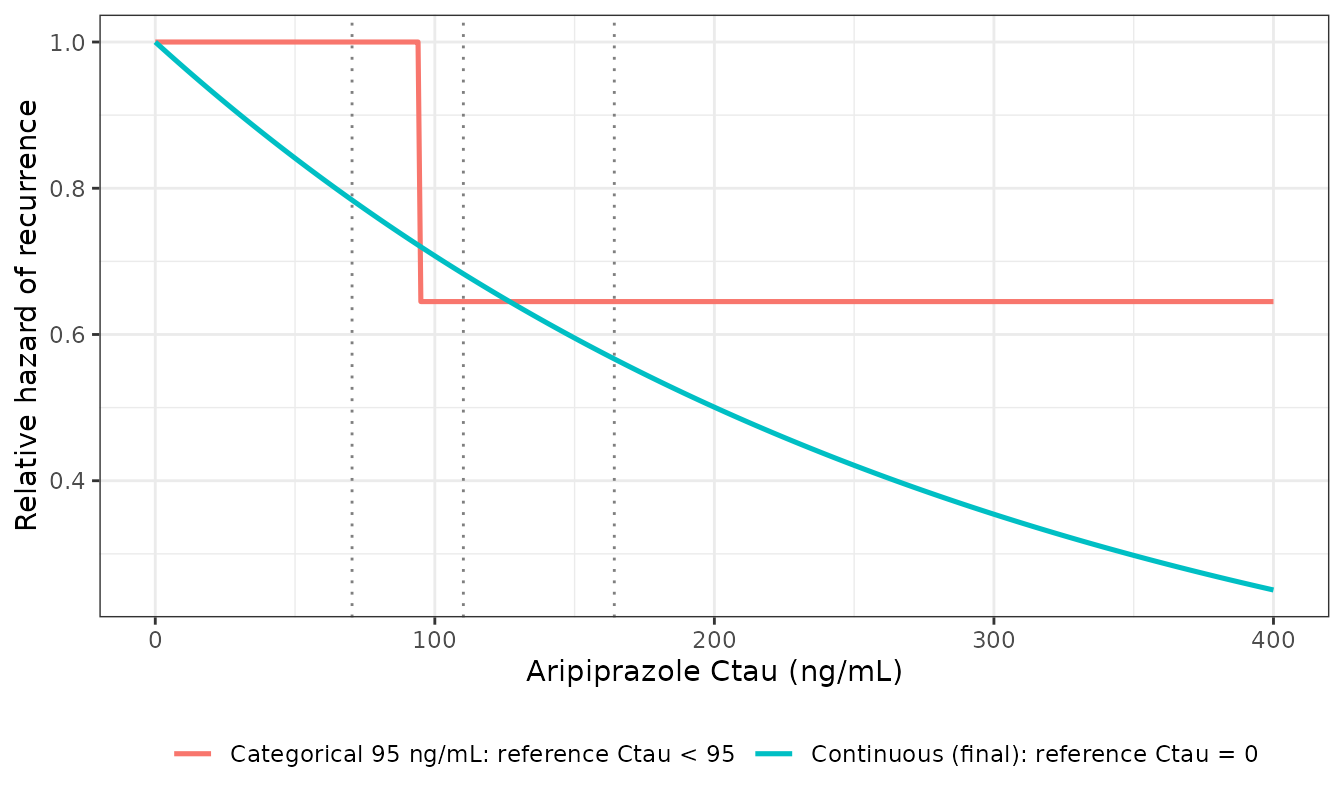
Relative hazard of recurrence of any mood episode against aripiprazole Ctau for the continuous (final) and categorical Wang 2025 models. Dotted lines mark the pooled Ctau quartile edges printed in the Figure 2 legend of Wang 2025.
The two models agree in direction but differ in what they say about patients above the threshold. Across the inter-quartile range of Ctau (70 to 164 ng/mL), the continuous model’s hazard falls to 0.723 times its value at the lower edge. The categorical model applies its single 0.645 step at 95 ng/mL and nothing beyond.
B. The exposure driver: reproducing Ctau with the upstream PK model
CTROUGH is an input to both models. Wang 2025 generated
it from each patient’s recorded dosing history and empirical-Bayes
parameters under the Wang 2022 PK model. The individual records are not
published. Below, a virtual trial is run through
Wang_2022_aripiprazole with the protocol’s dosing schedule,
and its predicted Ctau is compared with the published summaries. This
checks that the column a user would generate with the library’s PK model
lies on the same scale as the one these coefficients were fitted on.
# rxSetSeed() fixes rxode2's draws within one rxode2 build. The assertions
# below are on means and central quantiles, never on cohort extremes.
set.seed(20251101)
rxode2::rxSetSeed(20251101)

nPerArm <- 200L
bmiMean <- 30.2
bmiSd   <- 7.2
bmiSdlog <- sqrt(log(1 + (bmiSd / bmiMean)^2))

makeSubjects <- function(n, idOffset, arm) {
  tibble::tibble(
    id = idOffset + seq_len(n),
    arm = arm,
    SEXF = as.numeric(stats::runif(n) < 0.574),
    BMI = stats::rlnorm(n, log(bmiMean) - bmiSdlog^2 / 2, bmiSdlog),
    # 12 poor metabolisers among the 393 with a known phenotype (Table S3).
    CYP2D6_PM = as.numeric(stats::runif(n) < 12 / 393),
    CONMED_CYP2D6_INH = 0,
    CONMED_CYP3A4_INH = 0,
    STUDY_ARI_PHASE3 = 1,
    oralPhaseC = ifelse(stats::runif(n) < 0.5, 10, 15)
  )
}
subjects <- dplyr::bind_rows(
  makeSubjects(nPerArm, 0L, "AOM 400 mg"),
  makeSubjects(nPerArm, nPerArm, "Placebo")
)

tau   <- 672        # AOM dosing interval (h)
tC0   <- 42 * 24    # Phase C starts after 6 weeks of oral 15 mg QD (Phase B)
tD0   <- tC0 + 4 * tau  # first Phase D injection, after 4 Phase C AOM doses
tCtau <- tD0 + tau      # the Ctau landmark

# Oral doses use rate = -1 so the model's zero-order input R1 applies; AOM
# doses are bolus records into depot2. The placebo arm receives no Phase D
# dose. Observations are on the central ODE state.
doses <- dplyr::bind_rows(
  subjects |> dplyr::mutate(time = 0, amt = 15, cmt = "depot", rate = -1,
                            ii = 24, addl = 41L),
  subjects |> dplyr::mutate(time = tC0, amt = oralPhaseC, cmt = "depot",
                            rate = -1, ii = 24, addl = 13L),
  subjects |> dplyr::mutate(time = tC0, amt = 400, cmt = "depot2", rate = 0,
                            ii = tau, addl = 3L),
  subjects |> dplyr::filter(arm == "AOM 400 mg") |>
    dplyr::mutate(time = tD0, amt = 400, cmt = "depot2", rate = 0, ii = 0,
                  addl = 0L)
) |>
  dplyr::mutate(evid = 1L)
obs <- subjects |>
  tidyr::expand_grid(time = seq(tD0, tCtau, by = 24)) |>
  dplyr::mutate(amt = 0, cmt = "central", rate = 0, ii = 0, addl = 0L,
                evid = 0L)
events <- dplyr::bind_rows(doses, obs) |>
  dplyr::select(-oralPhaseC) |>
  dplyr::arrange(id, time, dplyr::desc(evid))

stopifnot(
  !anyDuplicated(events[events$evid == 0L, c("id", "time")]),
  nPerArm <= 200L
)
modPk <- readModelDb("Wang_2022_aripiprazole")
simPk <- as.data.frame(rxode2::rxSolve(modPk, events = events, keep = "arm",
                                       returnType = "data.frame"))
ctau <- simPk |>
  dplyr::filter(time == tCtau) |>
  dplyr::transmute(id, arm, CTROUGH = Cc)
stopifnot(nrow(ctau) == 2L * nPerArm)
ctauArm <- ctau |>
  dplyr::group_by(arm) |>
  dplyr::summarise(mean = mean(CTROUGH), sd = stats::sd(CTROUGH),
                   .groups = "drop") |>
  dplyr::mutate(pubMean = c(170.5, 78.7), pubSd = c(71.6, 36.1),
                pctDiff = 100 * (mean - pubMean) / pubMean)
ctauArm |>
  dplyr::mutate(dplyr::across(c(mean, sd, pctDiff), \(x) round(x, 1))) |>
  dplyr::rename("Arm" = arm, "Simulated mean" = mean, "Simulated SD" = sd,
                "Published mean" = pubMean, "Published SD" = pubSd,
                "Mean difference (%)" = pctDiff) |>
knitr::kable(caption = "Ctau by arm: virtual trial vs Wang 2025 Results and Table 1 (ng/mL).")| Arm | Simulated mean | Simulated SD | Published mean | Published SD | Mean difference (%) |
|---|---|---|---|---|---|
| AOM 400 mg | 177.1 | 85.8 | 170.5 | 71.6 | 3.9 |
| Placebo | 86.8 | 54.9 | 78.7 | 36.1 | 10.3 |
pooledQ <- stats::quantile(ctau$CTROUGH, c(0.25, 0.5, 0.75))
qTable <- tibble::tibble(
  quantity = c("25th percentile", "Median", "75th percentile",
               "Fraction below 95 ng/mL"),
  simulated = c(unname(pooledQ), mean(ctau$CTROUGH < 95)),
  published = c(70.39, 110.21, 164.2, 111 / 265)
) |>
  dplyr::mutate(pctDiff = 100 * (simulated - published) / published)
qTable |>
  dplyr::mutate(dplyr::across(c(simulated, published, pctDiff),
                              \(x) signif(x, 3))) |>
  dplyr::rename("Pooled Ctau" = quantity, "Virtual trial" = simulated,
                "Wang 2025" = published, "Difference (%)" = pctDiff) |>
knitr::kable(caption = "Pooled Ctau quartiles (Figure 2 legend) and the share below 95 ng/mL (Figure 3: 111 of 265).")| Pooled Ctau | Virtual trial | Wang 2025 | Difference (%) |
|---|---|---|---|
| 25th percentile | 75.200 | 70.400 | 6.83 |
| Median | 114.000 | 110.000 | 3.72 |
| 75th percentile | 169.000 | 164.000 | 3.15 |
| Fraction below 95 ng/mL | 0.408 | 0.419 | -2.71 |
stopifnot(
  # Structural: a mis-specified dose, interval or landmark (for example Ctau
  # read at the Phase D dose instead of 672 h later, which is identical for
  # the AOM arm but doubles the placebo value) moves these by tens of percent.
  all(abs(ctauArm$pctDiff) < 20),
  all(abs(qTable$pctDiff[1:3]) < 20),
  abs(qTable$simulated[4] - qTable$published[4]) < 0.10
)
The virtual trial lands within about 10% of every published summary. It sits slightly high, which matches the bias the paper reports when it applied this PK model to the bipolar data: a median population prediction error of -10.1% (observed below predicted) over all samples, and -2.0% in Phase D only (Table S4). The virtual trial also gives every AOM patient 400 mg, whereas 16.2% of the real cohort used 300 mg for part of the time.
C. PKNCA summary of the first double-blind interval
PKNCA does not apply to the Cox models themselves, which take no
dose. It does apply to the exposure interval that defines
CTROUGH. clast.obs over
[tD0, tD0 + 672 h] is Ctau. It must equal the Ctau
extracted above, which checks the landmark arithmetic.
concPk <- simPk |>
  dplyr::filter(!is.na(Cc)) |>
  dplyr::transmute(id, arm, time, Cc)
concObj <- PKNCA::PKNCAconc(concPk, Cc ~ time | arm + id)
intervals <- data.frame(start = tD0, end = tCtau, cmax = TRUE, cmin = TRUE,
                        cav = TRUE, clast.obs = TRUE)
ncaRes <- PKNCA::pk.nca(PKNCA::PKNCAdata(concObj, intervals = intervals))
#> No dose information provided, calculations requiring dose will return NA.
ncaWide <- as.data.frame(ncaRes) |>
  dplyr::select(arm, id, PPTESTCD, PPORRES) |>
  tidyr::pivot_wider(names_from = PPTESTCD, values_from = PPORRES)

ncaWide |>
  dplyr::group_by(arm) |>
  dplyr::summarise(dplyr::across(c(cmax, cmin, cav, clast.obs),
                                 \(x) round(stats::median(x), 1)),
                   .groups = "drop") |>
  dplyr::rename("Arm" = arm, "Cmax" = cmax, "Cmin" = cmin, "Cav" = cav,
                "Ctau (clast.obs)" = clast.obs) |>
knitr::kable(caption = "Median NCA over the first Phase D interval (ng/mL), virtual trial.")| Arm | Cmax | Cmin | Cav | Ctau (clast.obs) |
|---|---|---|---|---|
| AOM 400 mg | 251.3 | 153.3 | 212.3 | 159.2 |
| Placebo | 150.3 | 78.4 | 107.8 | 78.4 |
chk <- dplyr::inner_join(ncaWide, ctau, by = c("arm", "id"))
stopifnot(
  nrow(chk) == 2L * nPerArm,
  # Same simulated values, so the agreement is exact up to floating point.
  max(abs(chk$clast.obs - chk$CTROUGH)) < 1e-8
)
In the placebo arm, the interval minimum is the Ctau itself: the concentration only washes out. In the AOM arm, the median interval minimum lies a few percent below the median Ctau. For this formulation, the end-of-interval value is close to the interval minimum but not identical to it.
D. Relative hazard across the virtual trial
ctau$hrCont <- erEval(modCont, ctau$CTROUGH)
ctau$hrCut  <- erEval(modCut, ctau$CTROUGH)

ctau |>
  dplyr::group_by(arm) |>
  dplyr::summarise(
    `Median Ctau (ng/mL)` = round(stats::median(CTROUGH), 1),
    `Geometric mean hr, continuous` = signif(exp(mean(log(hrCont))), 3),
    `Share at or above 95 ng/mL` = round(mean(CTROUGH >= 95), 2),
    .groups = "drop"
  ) |>
  dplyr::rename("Arm" = arm) |>
knitr::kable()| Arm | Median Ctau (ng/mL) | Geometric mean hr, continuous | Share at or above 95 ng/mL |
|---|---|---|---|
| AOM 400 mg | 159.2 | 0.542 | 0.86 |
| Placebo | 78.4 | 0.741 | 0.32 |
ggplot(ctau, aes(CTROUGH, fill = arm)) +
  geom_histogram(binwidth = 20, alpha = 0.6, position = "identity",
                 boundary = 0) +
  geom_vline(xintercept = 95, linetype = "dashed") +
  labs(x = "Simulated aripiprazole Ctau (ng/mL)", y = "Patients", fill = NULL) +
  theme_bw() +
  theme(legend.position = "bottom")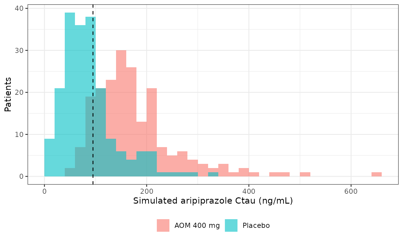
Distribution of simulated Ctau by arm, with the 95 ng/mL threshold of the categorical model. Compare with the pooled quartile edges of Wang 2025 Figure 2 (70.39, 110.21 and 164.2 ng/mL).
At the arm means, the continuous model gives the AOM arm a hazard about 0.73 times that of the placebo arm, from the published means 170.5 and 78.7 ng/mL. This is a much smaller contrast than the observed recurrence fractions (26.5% vs 51.1%) suggest. Part of the reason is that the single Ctau value is fixed per patient: in the placebo arm, exposure keeps falling after the landmark and the model cannot see it. Readers who want the treatment-arm contrast should not read it off these models.
Assumptions and deviations
-
No baseline hazard. Both models are semiparametric
Cox regressions. The baseline survival
S0(t)is unspecified by the method, and Wang 2025 does not report it. The models therefore return the relative hazard only, and Figure 3 (the survival VPC) cannot be reproduced. The maintainers did not build a parametric baseline from the Kaplan-Meier curves in Figures 2 and 3, because it would not come from the fit. -
The categorical HR is printed, its coefficient is
not.
e_ctrough_cut_hazislog(0.6450) = -0.4385. The log-scale midpoint of the printed 95% CI, -0.4386, confirms it. -
The 95 ng/mL threshold is fixed. It was carried
over from the schizophrenia analysis and tested, not estimated, so it is
wrapped in
fixed(). -
Screened covariates. Age, BMI, baseline MADRS,
baseline YMRS, sex and race were tested in a full model with backward
elimination (P < 0.01 to retain), and none was retained. No estimates
are reported. They are listed in
covariatesDataExcludedof the continuous model for provenance. That list names the YMRS scoreSCORE_YMRS, after the registeredSCORE_MADRS. The name is not a registered canonical and is documentation only. - Virtual-trial design, used for Section B only. It has 6 weeks of oral 15 mg QD (Phase B), then 4 open-label AOM 400 mg doses with oral 10 or 15 mg for the first 14 days (Phase C, the protocol minimum). The AOM arm then gets the first Phase D injection, and Ctau is read 672 h later. BMI is log-normal with the Table S5 mean and SD. The female share is 57.4%. The CYP2D6 poor-metaboliser share is 12/393 among the known phenotypes, and no patient takes a CYP inhibitor. The real Phase C lasted 12-28 weeks, and 16.2% of patients stepped down to 300 mg. The trial’s $MIX assignment of unknown CYP2D6 phenotypes is not reproduced.
- Table 1 placebo Ctau row is internally inconsistent. Table 1 gives the placebo arm’s mean (SD) Ctau as 16.4 (42.6) ng/mL for censored patients (n = 65) and 52.6 (58.6) ng/mL for patients with an event (n = 68), but 78.7 (36.1) ng/mL overall. The overall figure is larger than both subgroup means, so the three cannot all be right. The overall 78.7 ng/mL is repeated in the Results text, and it agrees with the washout predicted by the PK model (Section B). So Section B compares against the overall values. The AOM row is also not exactly self-consistent: the count-weighted mean of 187.2 and 163.3 is 180.9, against 170.5 printed. Only the printed overall means are used.
- Time unit. The models have no time dependence. The source analysis measured follow-up in days from randomisation, up to about 380 days (Figures 1-3).