Model and source
#> ℹ parameter labels from comments will be replaced by 'label()'Citation: Chala A, Kitabi EN, Ahmed JH, Tadesse BT, Chaka TE, Makonnen E, Aklillu E. Genetic and non-genetic factors influencing efavirenz population pharmacokinetics among human immunodeficiency virus-1-infected children in Ethiopia. CPT Pharmacometrics Syst Pharmacol. 2023;12(6):783-794. doi:10.1002/psp4.12951.
Description: One-compartment population pharmacokinetic-pharmacogenetic model with first-order absorption for oral efavirenz in antiretroviral-naive HIV-1-infected Ethiopian children aged 3-16 years (Chala 2023). Apparent oral clearance CL/F carries five multiplicative covariate factors: allometric body weight (exponent fixed to 0.75, reference 22 kg), CYP2B66 (c.516G>T, rs3745274) heterozygous and homozygous genotype factors, an ABCB1 c.4036A>G (rs3842) A-allele-carrier factor, a genotype-gated autoinduction step (CL/F rises from week 12 in CYP2B61/1 and from week 8 in CYP2B61/6, with no change in 6/*6), and a two-class latent mixture in which 7.5% of children form a subpopulation with 3.5-fold lower CL/F. Apparent volume V/F scales linearly with weight (exponent fixed to 1). Absorption rate ka was not identifiable from the sparse design and is fixed to 0.776 1/h; interindividual variability on V/F and ka was likewise not identifiable and was fixed to zero, leaving CL/F as the only random effect.
Article: https://doi.org/10.1002/psp4.12951
Supplement (Appendix S1, the NONMEM control stream; Tables S1-S3; Figures S1-S3): https://europepmc.org/article/PMC/PMC10272302
Chala 2023 developed a one-compartment population pharmacokinetic
model with first-order absorption for oral efavirenz in
antiretroviral-therapy-naive HIV-1-infected Ethiopian children. Apparent
oral clearance CL/F carries five multiplicative factors – allometric
body weight, CYP2B6*6 genotype, ABCB1
c.4036A>G (rs3842) genotype, a genotype-gated autoinduction step, and
a latent two-class mixture – while apparent volume V/F scales linearly
with weight. Absorption rate ka and the interindividual
variability on V/F and ka could not be identified from the
sparse design and were fixed.
Population
One hundred combination-antiretroviral-therapy-naive children aged 3-16 years were enrolled from seven hospital ART centres in the Oromia and Southern Nations, Nationalities and Peoples regional states of Ethiopia (Chala 2023 Table 1). Median age was 9 years (IQR 6-13), median weight 22.05 kg (IQR 16.8-28.25) and 42% were female. Baseline liver and renal function were broadly normal (median eGFR 95.5 mL/min/1.73m^2, median albumin 3.8 mg/dL) and CD4 counts were immunocompetent (median 330 cells/dL); 15% had active pulmonary tuberculosis and 69% were receiving cotrimoxazole prophylaxis.
Genotype frequencies (Table 1) are the ones that make this cohort
informative: CYP2B6*6 was *1/*1 in 45%,
*1/*6 in 45% and *6/*6 in 8%, and
ABCB1 c.4036A>G (rs3842) was G/G in 17% versus G/A or
A/A in 80%.
554 efavirenz plasma concentrations were collected over one year in a
two-arm design: 13 children gave rich samples at 0, 2.5, 16 and 24 h
after the first dose (9 repeated at week 8), and 87 children
gave a single mid-dose sample 8-16 h post dose at weeks 4, 8, 12, 24 and
48. That sparseness is the reason ka and two of the three
IIV terms are fixed rather than estimated.
The same information is available programmatically via
rxode2::rxode(readModelDb("Chala_2023_efavirenz"))$population.
Source trace
Every ini() entry carries an in-file comment naming its
source location in
inst/modeldb/specificDrugs/Chala_2023_efavirenz.R. They are
collected here for review. Point estimates are taken from supplement
Table S3 run32 – the final run, the only one carrying
all twelve thetas – which prints the same values as main-text Table 2 to
more significant figures.
| Equation / parameter | Value | Source location |
|---|---|---|
lcl (CL/F at the 22 kg reference) |
4.30 L/h | Table 2 CL (L/h) 4.30 (RSE 13%, bootstrap 3.20-5.30);
Equation 1 4.3(CLpop)
|
lvc (V/F at the 22 kg reference) |
123.80 L | Table 2 V c (L) 123.80 (RSE 10%, bootstrap
103.30-163.80) |
lka |
0.776 1/h, fixed | Table 2 K a (/h) 0.78 + footnote “Fixed to this value”;
unrounded value in Results para. 7 and abstract; Appendix S1
$THETA (0.776) FIX ; KA
|
e_wt_cl |
0.75, fixed | Results para. 3 step 3 CLi = CLpop * (WT/22)^0.75;
Discussion para. 3 “fixed to theoretical values”; Appendix S1
(WT/22)**0.75
|
e_wt_vc |
1, fixed | Results para. 3 step 3 Vi = Vpop * (WT/22); Appendix S1
TVV = THETA(2)*(WT/22)
|
e_cyp2b6_6het_cl |
0.7245 | Table 2 “Fraction of typical CL … CYP2B61/6” 0.72; Table S3
run32 CP2B6S1S6
|
e_cyp2b6_6hom_cl |
0.2823 | Table 2 “Fraction of typical CL … CYP2B66/6” 0.28; Table S3
run32 CP2B6S6S6
|
e_snp_abcb1_rs3842_a_cl |
1.452 | Table 2 “Fold of typical CL … ABCB1.rs3842 G/A or A/A” 1.45; Table
S3 run32 ABCB1RS3842
|
e_autoind_cyp2b6_6wt_cl |
0.1235 | Table 2 “Proportional increase in CL from >= 12-weeks …
CYP2B61/1” 0.12; Table S3 run32
CP2B6S1S1WEEK12
|
e_autoind_cyp2b6_6het_cl |
0.2298 | Table 2 “Proportional increase in CL from >= 8weeks …
CYP2B61/6” 0.23; Table S3 run32
CP2B6S1S6WEEK8
|
e_mix_slow_elim_efv_cl |
0.2829 | Table 2 “Fraction of typical of CL for the subpopulation” 0.28;
Table S3 run32 MIXPOP
|
| mixture class probability | 0.07511 | Table 2 “Proportion of an unknown subpopulation” 0.075; Appendix S1
$MIX ... P(1) = THETA(11). Carried in
covariateData$MIX_SLOW_ELIM_EFV$notes, not in
ini()
|
etalcl |
0.118127 | Table 2 “Interindividual variability for CL (%CV)” 35.4; Table S3
run32 IIVCL 0.3541. omega^2 = log(CV^2 + 1)
per Methods para. 2 (CV% = 100 * sqrt(exp(omega^2) - 1)).
Scale confirmed by the same row’s bootstrap 0.105 (95% CI 0.05-0.169),
which is on the variance scale and brackets 0.118127 |
propSd |
0.4969 | Table 2 “Proportional residual error (%CV)” 50%; Table S3 run32
PROP
|
addSd |
0.00028 ug/mL, fixed | Appendix S1 $THETA (0.00028) FIX ; ADD. Not reported in
main-text Table 2 – see Errata |
| CL/F equation (product of indicator-powered factors) | n/a | Equation 1; Appendix S1
TVCL = THETA(1) * CP2B6CL * ABCB1RS3842CL * (WT/22)**0.75 * CLWKCP2B61 * CLWKCP2B62 * CLMIX
|
d/dt(depot), d/dt(central)
|
n/a | Results para. 2 “one-compartment model parameterized in oral
clearance, oral volume of distribution and absorption rate constant”;
Appendix S1 $SUBROUTINE ADVAN2 TRANS=2
|
| Residual error form | n/a | Appendix S1
$ERROR: W = SQRT(ADD**2 + PROP**2*IPRED**2); Y = IPRED + W*ERR(1)
with $SIGMA 1 FIX
|
Structural verification: reproducing Equation 1
Chala 2023 Equation 1 writes individual clearance as a product of factors, each raised to a 0/1 indicator power:
CLi = ( 4.3 * (WT/22)^0.75 * 0.72^f1 * 0.28^f2 * 1.45^f3
            * 1.12^f4 * 1.23^f5 * 0.28^f6 ) * exp(eta)
The checks below are deterministic – they compare typical values from the packaged model against closed-form arithmetic, so exact tolerances are correct here and are deliberately tight.
mod <- readModelDb("Chala_2023_efavirenz")
mod_typical <- rxode2::zeroRe(mod)
#> ℹ parameter labels from comments will be replaced by 'label()'

# One scenario per row. `week` is weeks on efavirenz-based ART; the canonical
# T_FIRSTDOSE column carries it in hours (168 h per week).
scen <- tibble::tribble(
  ~scenario,                              ~WT,  ~cyp,  ~aCar, ~week, ~mix,
  "Reference: 22 kg, *1/*1, G/G, week 1",  22,     0L,     0L,     1,   0L,
  "CYP2B6 *1/*6",                          22,     1L,     0L,     1,   0L,
  "CYP2B6 *6/*6",                          22,     2L,     0L,     1,   0L,
  "ABCB1 rs3842 G/A or A/A",               22,     0L,     1L,     1,   0L,
  "*1/*1 at week 8 (no step yet)",         22,     0L,     0L,     8,   0L,
  "*1/*1 at week 12 (step applies)",       22,     0L,     0L,    12,   0L,
  "*1/*6 at week 4 (no step yet)",         22,     1L,     0L,     4,   0L,
  "*1/*6 at week 8 (step applies)",        22,     1L,     0L,     8,   0L,
  "*6/*6 at week 48 (never steps)",        22,     2L,     0L,    48,   0L,
  "Latent slow-eliminator subpopulation",  22,     0L,     0L,     1,   1L,
  "70 kg adult-size extrapolation",        70,     0L,     0L,     1,   0L,
  "10 kg child",                           10,     0L,     0L,     1,   0L
)

# Closed-form Equation 1 (typical value; exp(eta) = 1 under zeroRe).
eq1_cl <- function(WT, cyp, aCar, week, mix) {
  4.30 * (WT / 22)^0.75 *
    0.7245^(cyp == 1L) *
    0.2823^(cyp == 2L) *
    1.452^aCar *
    (1 + 0.1235)^(cyp == 0L & week >= 12) *
    (1 + 0.2298)^(cyp == 1L & week >= 8) *
    0.2829^mix
}
eq1_vc <- function(WT) 123.80 * (WT / 22)

# Build a one-dose / one-observation event table per scenario and solve.
ev_struct <- scen |>
  mutate(id = dplyr::row_number()) |>
  tidyr::crossing(tibble(time = c(0, 12), evid = c(1L, 0L),
                         amt = c(300, NA_real_), cmt = c("depot", "central"))) |>
  mutate(
    SNP_CYP2B6_RS3745274_T_COUNT = cyp,
    SNP_ABCB1_RS3842_A_CARRIER   = aCar,
    MIX_SLOW_ELIM_EFV            = mix,
    T_FIRSTDOSE                  = week * 168
  ) |>
  arrange(id, time, desc(evid)) |>
  as.data.frame()

sim_struct <- rxode2::rxSolve(mod_typical, ev_struct,
                              keep = c("scenario", "WT", "cyp", "aCar",
                                       "week", "mix")) |>
  as.data.frame()
#> ℹ omega/sigma items treated as zero: 'etalcl'
#> Warning: multi-subject simulation without without 'omega'

struct_tab <- sim_struct |>
  group_by(scenario, WT, cyp, aCar, week, mix) |>
  summarise(cl_model = mean(cl), vc_model = mean(vc), .groups = "drop") |>
  mutate(
    cl_closed = eq1_cl(WT, cyp, aCar, week, mix),
    vc_closed = eq1_vc(WT),
    cl_pct    = 100 * (cl_model - cl_closed) / cl_closed,
    vc_pct    = 100 * (vc_model - vc_closed) / vc_closed
  ) |>
  arrange(match(scenario, scen$scenario))

# Deterministic identity: the packaged model must reproduce Equation 1 to
# machine precision. This is NOT a cohort statistic, so an exact bound is the
# right gate (the headroom rule applies to simulated cohorts, which vary with
# the solver thread count, and explicitly not to closed-form identities).
stopifnot(
  max(abs(struct_tab$cl_pct)) < 1e-8,
  max(abs(struct_tab$vc_pct)) < 1e-8
)

struct_tab |>
  select(scenario, cl_model, cl_closed, cl_pct, vc_model, vc_closed) |>
  dplyr::rename(
    "Scenario"              = scenario,
    "CL/F model (L/h)"      = cl_model,
    "CL/F Equation 1 (L/h)" = cl_closed,
    "Difference (%)"        = cl_pct,
    "V/F model (L)"         = vc_model,
    "V/F closed form (L)"   = vc_closed
  ) |>
  knitr::kable(
    digits  = c(0, 4, 4, 10, 3, 3),
    caption = "Typical CL/F and V/F from the packaged model against Chala 2023 Equation 1 evaluated by hand."
)| Scenario | CL/F model (L/h) | CL/F Equation 1 (L/h) | Difference (%) | V/F model (L) | V/F closed form (L) |
|---|---|---|---|---|---|
| Reference: 22 kg, 1/1, G/G, week 1 | 4.3000 | 4.3000 | 0 | 123.800 | 123.800 |
| CYP2B6 1/6 | 3.1154 | 3.1153 | 0 | 123.800 | 123.800 |
| CYP2B6 6/6 | 1.2139 | 1.2139 | 0 | 123.800 | 123.800 |
| ABCB1 rs3842 G/A or A/A | 6.2436 | 6.2436 | 0 | 123.800 | 123.800 |
| 1/1 at week 8 (no step yet) | 4.3000 | 4.3000 | 0 | 123.800 | 123.800 |
| 1/1 at week 12 (step applies) | 4.8311 | 4.8310 | 0 | 123.800 | 123.800 |
| 1/6 at week 4 (no step yet) | 3.1154 | 3.1153 | 0 | 123.800 | 123.800 |
| 1/6 at week 8 (step applies) | 3.8313 | 3.8313 | 0 | 123.800 | 123.800 |
| 6/6 at week 48 (never steps) | 1.2139 | 1.2139 | 0 | 123.800 | 123.800 |
| Latent slow-eliminator subpopulation | 1.2165 | 1.2165 | 0 | 123.800 | 123.800 |
| 70 kg adult-size extrapolation | 10.2441 | 10.2441 | 0 | 393.909 | 393.909 |
| 10 kg child | 2.3804 | 2.3804 | 0 | 56.273 | 56.273 |
Two rows above are independent checks rather than restatements of the same arithmetic:
- The 70 kg extrapolation is the one number Chala
2023 reports on a scale other than its own 22 kg reference. Discussion
paragraph 5 states the typical value as
10.24 (7.6-12.6) L/h/70 kg, contrasting it with Bienczak et al.’s 21.6 L/h/70 kg. That figure is not used anywhere in building the model file, so reproducing it tests the clearance estimate, the reference weight and the allometric exponent jointly. - The
*6/*6row tests the abstract’s claim that clearance is “reduced by … 72%” inCYP2B6*6/*6, and the*1/*6row the companion “reduced by 28%”.
cl70 <- struct_tab$cl_model[struct_tab$scenario == "70 kg adult-size extrapolation"]
pub70 <- 10.24  # Chala 2023 Discussion para. 5: "typical value (95% CI) = 10.24 [7.6-12.6] L/h/70 kg"

reduction <- struct_tab |>
  filter(scenario %in% c("CYP2B6 *1/*6", "CYP2B6 *6/*6")) |>
  mutate(pct_reduction = 100 * (1 - cl_model / 4.30))

claims <- tibble::tibble(
  Claim = c(
    "CL/F at 70 kg = 10.24 L/h (Discussion para. 5)",
    "CL/F reduced by 28% in CYP2B6*1/*6 (abstract)",
    "CL/F reduced by 72% in CYP2B6*6/*6 (abstract)"
  ),
  Units     = c("L/h", "% reduction", "% reduction"),
  Published = c(10.24, 28, 72),
  Model     = c(cl70, reduction$pct_reduction[1], reduction$pct_reduction[2])
) |>
  mutate(
    `Difference (relative %)` = 100 * (Model - Published) / Published,
    `Difference (absolute)`   = Model - Published
  )

# These are deterministic (zeroRe) closed-form values, so the only residual is
# the paper's own rounding -- but the two kinds of claim need different gates.
#
# The 70 kg clearance is printed to four significant figures, so a relative
# bound is right: 0.5% admits the rounding while a wrong allometric exponent or
# reference weight (which move it by tens of percent) still fails.
#
# The two "reduced by N%" claims come from fractions printed to two decimal
# places (0.72 and 0.28) and then rounded to a whole percent, so the honest gate
# is an ABSOLUTE bound in percentage points, not a relative one: the unrounded
# 0.7245 gives a 27.55% reduction against a published "28%", which is 0.45
# percentage points of rounding but 1.6% in relative terms. One percentage point
# covers the rounding; a mis-transcribed genotype factor moves these by tens of
# percentage points and still fails.
stopifnot(
  abs(claims$`Difference (relative %)`[1]) < 0.5,
  max(abs(claims$`Difference (absolute)`[2:3])) < 1
)

knitr::kable(claims, digits = 3,
caption = "Model against the three CL/F statements Chala 2023 makes outside its own parameter table.")| Claim | Units | Published | Model | Difference (relative %) | Difference (absolute) |
|---|---|---|---|---|---|
| CL/F at 70 kg = 10.24 L/h (Discussion para. 5) | L/h | 10.24 | 10.244 | 0.040 | 0.004 |
| CL/F reduced by 28% in CYP2B61/6 (abstract) | % reduction | 28.00 | 27.550 | -1.607 | -0.450 |
| CL/F reduced by 72% in CYP2B66/6 (abstract) | % reduction | 72.00 | 71.770 | -0.319 | -0.230 |
Genotype-gated autoinduction
Efavirenz induces its own metabolism. Chala 2023 Results paragraph 5
reports that the induction becomes statistically significant at a
different treatment week in each CYP2B6*6
genotype: from week 12 in *1/*1, from week 8 in
*1/*6, and not at all in *6/*6.
weeks <- c(0, 1, 4, 8, 12, 24, 48)
auto <- tidyr::crossing(week = weeks, cyp = 0:2) |>
  mutate(
    Genotype = factor(cyp, 0:2,
                      c("CYP2B6 *1/*1", "CYP2B6 *1/*6", "CYP2B6 *6/*6")),
    cl = eq1_cl(22, cyp, 0L, week, 0L)
  ) |>
  group_by(Genotype) |>
  mutate(`CL/F relative to week 1` = cl / cl[week == 1]) |>
  ungroup()

ggplot(auto, aes(week, `CL/F relative to week 1`, colour = Genotype)) +
  geom_step(direction = "hv", linewidth = 0.9) +
  geom_point(size = 2) +
  scale_x_continuous(breaks = weeks) +
  labs(x = "Weeks on efavirenz-based ART", y = "CL/F relative to week 1",
       title = "Genotype-gated autoinduction of efavirenz CL/F",
       caption = "Reproduces Chala 2023 Results paragraph 5 / Table 2 rows 9-10.") +
  theme_bw()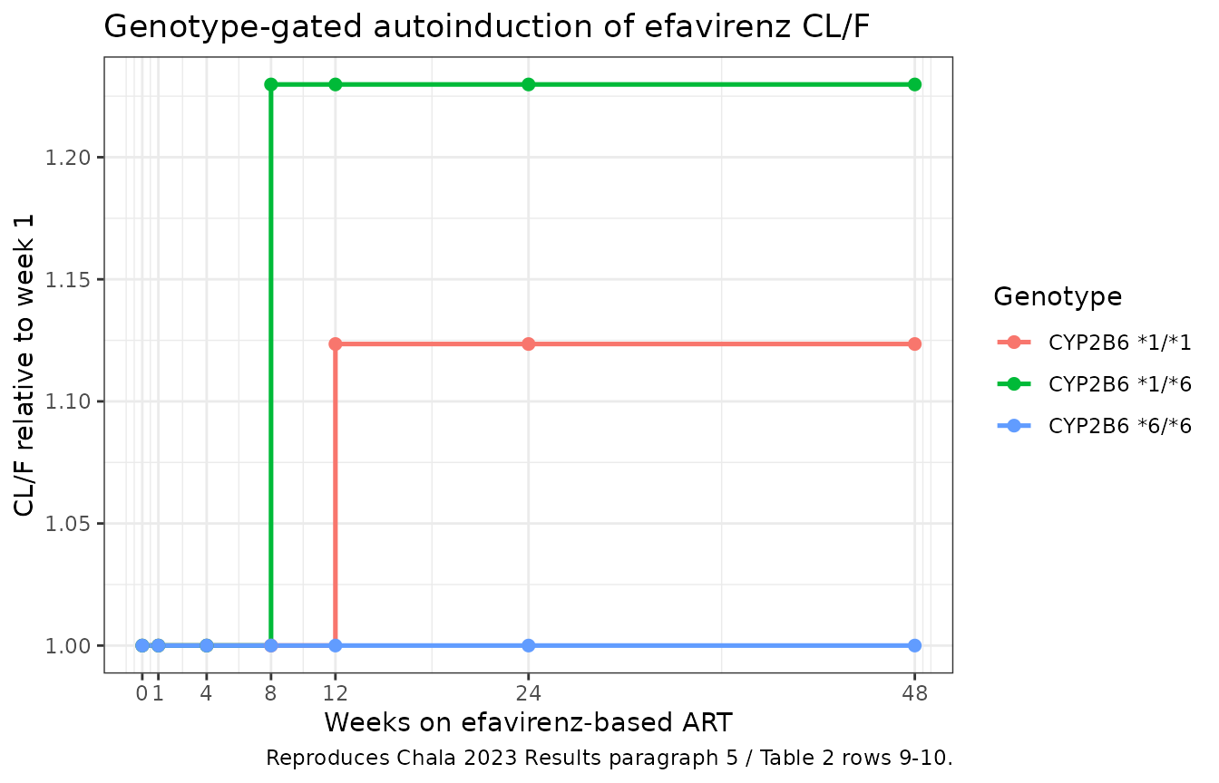
# Deterministic step sizes straight from Table 2.
step <- auto |>
  select(Genotype, week, `CL/F relative to week 1`) |>
  tidyr::pivot_wider(names_from = week, values_from = `CL/F relative to week 1`,
                     names_prefix = "wk")
stopifnot(
  isTRUE(all.equal(step$wk8[1],  1.0000, tolerance = 1e-10)),  # *1/*1 no step at week 8
  isTRUE(all.equal(step$wk12[1], 1.1235, tolerance = 1e-10)),  # *1/*1 steps at week 12
  isTRUE(all.equal(step$wk4[2],  1.0000, tolerance = 1e-10)),  # *1/*6 no step at week 4
  isTRUE(all.equal(step$wk8[2],  1.2298, tolerance = 1e-10)),  # *1/*6 steps at week 8
  isTRUE(all.equal(step$wk48[3], 1.0000, tolerance = 1e-10))   # *6/*6 never steps
)
Virtual cohort
Original observed data are not publicly available. The cohort below
approximates the Monte-Carlo design Chala 2023 used for its Figure 3
(Methods, final paragraph): virtual children stratified by weight band,
with CYP2B6*6 genotype held fixed within each stratum,
ABCB1 rs3842 drawn at 80% G/A-or-A/A and the latent
slow-eliminator class drawn at the estimated 7.5% probability.
Doses are the modal dose actually received in each weight band, from supplement Table S1. Only the four bands whose modal dose agrees with the SUSTIVA label are simulated; the 25-32.5 kg and 32.5-40 kg bands are omitted because their modal received dose (600 mg) is above the label recommendation – Chala 2023 notes that “a few individuals received higher doses than recommended”, and including those bands would inflate the exposure claims below rather than test them.
# set.seed() fixes the covariate draws below (they are drawn in R). It does NOT
# fix rxode2's eta draws, whose streams are partitioned per solver thread, so a
# CI runner draws different etas than this machine. Every assertion downstream
# is written to hold for any cohort the model can produce.
set.seed(20230612)

n_per_arm <- 100L  # 12 arms; well under the 200-per-arm cap

bands <- tibble::tribble(
  ~band,        ~wt_lo, ~wt_hi, ~dose_mg,
  "7.5-15 kg",     7.5,   15.0,   200,   # Table S1: 200 mg in 66.7% of the band
  "15-20 kg",     15.0,   20.0,   250,   # Table S1: 250 mg in 55.6%
  "20-25 kg",     20.0,   25.0,   300,   # Table S1: 300 mg in 61.1%
  ">40 kg",       40.0,   60.0,   600    # Table S1: 600 mg in 100%
) |>
  mutate(band = factor(band, levels = band))

genos <- tibble::tibble(
  cyp      = 0:2,
  Genotype = factor(c("CYP2B6 *1/*1", "CYP2B6 *1/*6", "CYP2B6 *6/*6"),
                    levels = c("CYP2B6 *1/*1", "CYP2B6 *1/*6", "CYP2B6 *6/*6"))
)

# Steady state at week 24 of therapy: 14 once-daily doses (t = 0, 24, ..., 312),
# then observations across the final interval. Efavirenz t1/2 here is about
# 20 h, so 13 days of dosing is well over 15 half-lives.
n_dose  <- 14L
tau     <- 24
t_last  <- (n_dose - 1L) * tau          # 312 h
wk_at_start <- 24                        # weeks on ART at the start of the window

subjects <- tidyr::crossing(bands, genos) |>
  mutate(arm = paste(band, Genotype, sep = " | ")) |>
  tidyr::uncount(n_per_arm) |>
  mutate(
    id   = dplyr::row_number(),
    WT   = runif(dplyr::n(), wt_lo, wt_hi),
    SNP_CYP2B6_RS3745274_T_COUNT = cyp,
    SNP_ABCB1_RS3842_A_CARRIER   = rbinom(dplyr::n(), 1L, 0.80),
    MIX_SLOW_ELIM_EFV            = rbinom(dplyr::n(), 1L, 0.075)
  )

dose_rows <- subjects |>
  tidyr::crossing(time = seq(0, t_last, by = tau)) |>
  mutate(evid = 1L, amt = dose_mg, cmt = "depot")

obs_rows <- subjects |>
  tidyr::crossing(time = seq(t_last, t_last + tau, by = 1)) |>
  mutate(evid = 0L, amt = NA_real_, cmt = "central")

events <- bind_rows(dose_rows, obs_rows) |>
  # T_FIRSTDOSE is treatment duration, not time after dose: it keeps rising
  # across the record and does not reset at each dosing event.
  mutate(T_FIRSTDOSE = wk_at_start * 168 + time) |>
  arrange(id, time, desc(evid)) |>
  as.data.frame()

# No id/time/evid record is repeated. Note the deliberate absence of `unique()`
# here: de-duplicating first would make the check vacuously true. The 312 h row
# appears twice by design (the last dose and the first observation of the
# window), which the `evid` column keeps distinct.
stopifnot(!anyDuplicated(events[, c("id", "time", "evid")]))Replicate Figure 3
Chala 2023 Figure 3 reports population summary statistics of the
efavirenz concentration 12 h after dose, by dosing weight band and
CYP2B6*6 genotype. Results paragraph 8 states three
findings, all reproduced below:
- “EFV concentrations at 12-h after dose are comparable across the dosing weight bands.”
- “subjects with
CYP2B6*6/*6have relatively higher EFV concentrations … with greater than 80% of those subjects having EFV concentrations greater than 4 ug/mL.” - “greater than 80% of subjects with
CYP2B6*1/*1orCYP2B6*1/*6who receive EFV dosing according to the SUSTIVA label, are predicted to have EFV concentration greater than or equal to 1 ug/mL.”
c12 <- sim |>
  filter(time == t_last + 12) |>
  select(id, arm, band, Genotype, WT, dose_mg, C12 = Cc)

stopifnot(nrow(c12) == nrow(subjects), !anyNA(c12$C12))

ggplot(c12, aes(band, C12, fill = Genotype)) +
  geom_boxplot(outlier.size = 0.5, position = position_dodge(width = 0.8)) +
  geom_hline(yintercept = c(1, 4), linetype = "dashed", colour = "grey30") +
  scale_y_log10() +
  labs(x = "Dosing weight band", y = "Efavirenz concentration 12 h post dose (ug/mL)",
       title = "Steady-state 12-h efavirenz concentration by weight band and CYP2B6*6 genotype",
       caption = paste("Replicates Figure 3 of Chala 2023. Dashed lines mark the 1 and",
                       "4 ug/mL thresholds discussed in the paper.")) +
  theme_bw() +
  theme(legend.position = "bottom")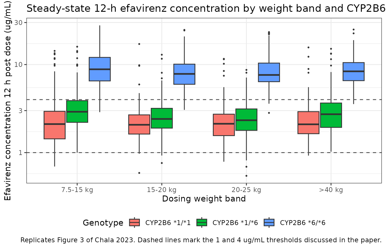
band_medians <- c12 |>
  group_by(Genotype, band) |>
  summarise(median_C12 = median(C12), .groups = "drop_last") |>
  summarise(band_spread = max(median_C12) / min(median_C12), .groups = "drop")

pct_over_4 <- c12 |>
  filter(Genotype == "CYP2B6 *6/*6") |>
  summarise(pct = 100 * mean(C12 > 4)) |>
  pull(pct)

pct_over_1 <- c12 |>
  filter(Genotype != "CYP2B6 *6/*6") |>
  summarise(pct = 100 * mean(C12 >= 1)) |>
  pull(pct)

fig3 <- tibble::tibble(
  Claim = c(
    "12-h concentrations comparable across weight bands (max/min of band medians, within genotype)",
    "% of CYP2B6*6/*6 subjects above 4 ug/mL",
    "% of CYP2B6*1/*1 or *1/*6 subjects at or above 1 ug/mL"
  ),
  `Chala 2023` = c("comparable", "> 80%", "> 80%"),
  Model = c(
    sprintf("%.2f-%.2f fold", min(band_medians$band_spread), max(band_medians$band_spread)),
    sprintf("%.1f%%", pct_over_4),
    sprintf("%.1f%%", pct_over_1)
  )
)

knitr::kable(fig3, caption = "Chala 2023 Figure 3 / Results paragraph 8 claims against the packaged model.")| Claim | Chala 2023 | Model |
|---|---|---|
| 12-h concentrations comparable across weight bands (max/min of band medians, within genotype) | comparable | 1.03-1.25 fold |
| % of CYP2B66/6 subjects above 4 ug/mL | > 80% | 96.8% |
| % of CYP2B61/1 or 1/6 subjects at or above 1 ug/mL | > 80% | 97.1% |
# Bounds chosen with headroom over what a cohort draw can move. The
# band-spread bound of 1.5 is a magnitude claim about "comparable", not a race
# between two noisy statistics; a mis-transcribed allometric exponent takes the
# 7.5-15 kg / >40 kg ratio well past 2. The two percentage bounds sit 5-10
# points below the paper's own ">80%" so a different eta draw cannot flip them,
# while a wrong genotype fold-factor (which moves these by tens of points)
# still fails them.
stopifnot(
  max(band_medians$band_spread) < 1.5,
  pct_over_4 > 70,
  pct_over_1 > 75
)
The CYP2B6*6/*6 stratum sits about three-and-a-half-fold
above the other two genotypes, which is the paper’s central clinical
message: on label dosing these children are systematically over-exposed
relative to the 1-4 ug/mL therapeutic range, and the Discussion proposes
an approximately three-fold dose reduction for them.
Both threshold claims are stated in the paper as lower bounds (“greater than 80%”), and the packaged model clears them with room to spare – around 97% on each. Part of that margin is a design difference rather than a model disagreement: the four weight bands simulated here are the label-consistent ones, whereas Chala 2023’s Figure 3 also spans the smallest weight bands and draws its virtual weights from NHANES rather than uniformly. The direction and the ordering across genotypes are what the replication establishes; the exact percentage is not a published number to match.
sim |>
  mutate(tad = time - t_last) |>
  group_by(tad, Genotype) |>
  summarise(Q05 = quantile(Cc, 0.05), Q50 = median(Cc),
            Q95 = quantile(Cc, 0.95), .groups = "drop") |>
  ggplot(aes(tad, Q50, colour = Genotype, fill = Genotype)) +
  geom_ribbon(aes(ymin = Q05, ymax = Q95), alpha = 0.18, colour = NA) +
  geom_line(linewidth = 0.9) +
  scale_y_log10() +
  labs(x = "Time after the last dose (h)", y = "Efavirenz concentration (ug/mL)",
       title = "Steady-state efavirenz profile by CYP2B6*6 genotype (all weight bands pooled)",
       caption = "Median with 5th-95th percentile band; week 24 of therapy.") +
  theme_bw() +
  theme(legend.position = "bottom")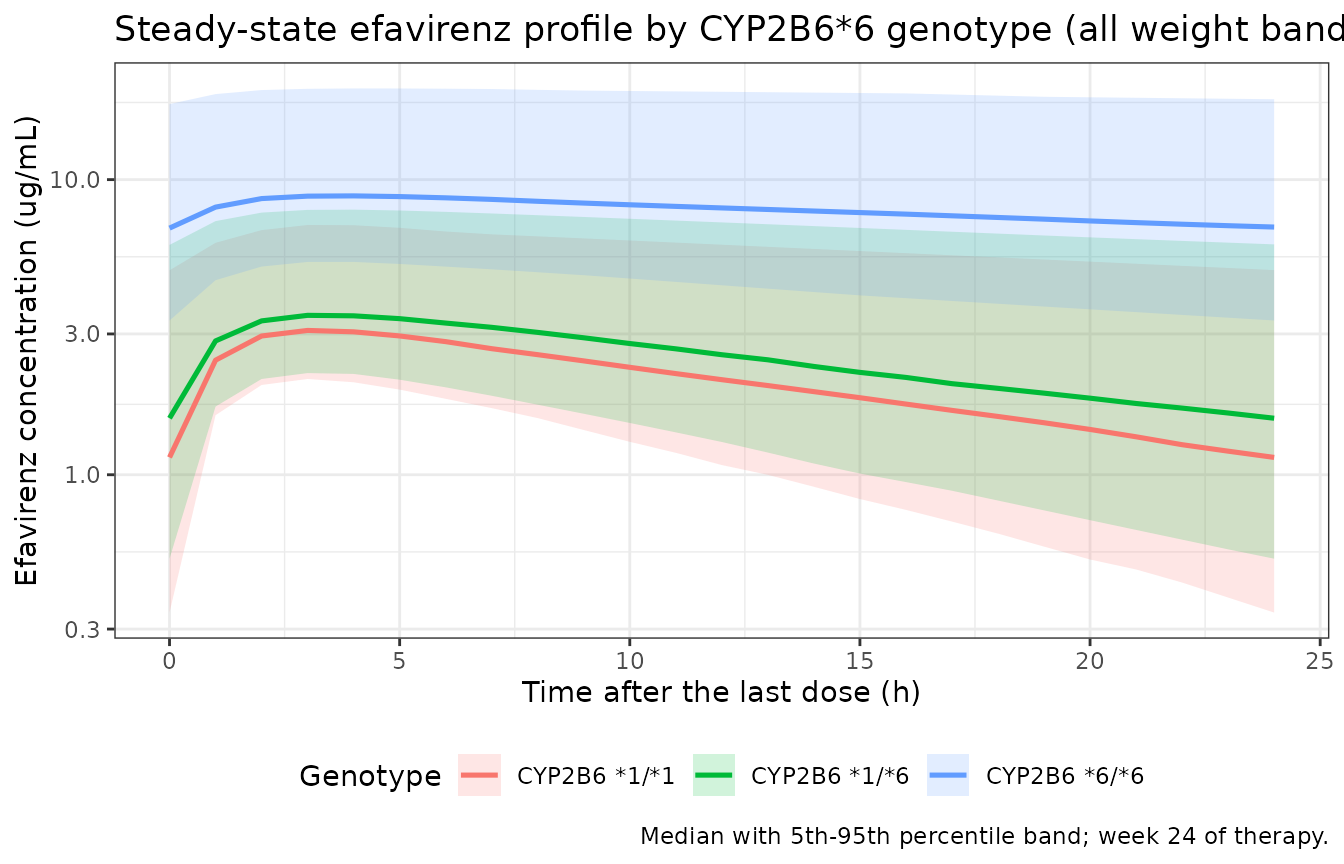
PKNCA validation
Chala 2023 reports no non-compartmental parameters – neither Cmax, Tmax, AUC nor half-life appears in the paper or the supplement – so there is nothing to compare a simulated NCA table against. The NCA below is therefore run against exact internal identities on a typical-value (no-IIV, no-residual-error) profile, which is a stricter gate than a 20%-tolerance comparison would be:
- at steady state,
AUC(0-tau) = Dose / (CL/F)exactly for a linear model; - the terminal half-life must equal
log(2) * (V/F) / (CL/F), becausekel(0.0347 1/h at the 22 kg reference) is far belowka = 0.776 1/hand no flip-flop occurs.
Note that the half-life is not constant across weight bands:
V/F scales with WT^1 and CL/F
with WT^0.75, so log(2) * V/F / (CL/F) grows
as WT^0.25 – from about 15 h in the smallest band to about
22 h in the largest.
nca_subj <- bands |>
  mutate(
    id  = dplyr::row_number(),
    WT  = (wt_lo + wt_hi) / 2,
    arm = paste0(band, " (", dose_mg, " mg)"),
    SNP_CYP2B6_RS3745274_T_COUNT = 0L,   # CYP2B6 *1/*1
    SNP_ABCB1_RS3842_A_CARRIER   = 0L,   # rs3842 G/G
    MIX_SLOW_ELIM_EFV            = 0L    # main population
  )

nca_events <- bind_rows(
  nca_subj |>
    tidyr::crossing(time = seq(0, t_last, by = tau)) |>
    mutate(evid = 1L, amt = dose_mg, cmt = "depot"),
  nca_subj |>
    tidyr::crossing(time = seq(t_last, t_last + tau, by = 0.25)) |>
    mutate(evid = 0L, amt = NA_real_, cmt = "central")
) |>
  mutate(T_FIRSTDOSE = wk_at_start * 168 + time) |>
  arrange(id, time, desc(evid)) |>
  as.data.frame()

sim_nca_raw <- rxode2::rxSolve(mod_typical, nca_events,
                               keep = c("arm", "dose_mg", "WT")) |>
  as.data.frame()
#> ℹ omega/sigma items treated as zero: 'etalcl'
#> Warning: multi-subject simulation without without 'omega'

# PKNCA input filter: `!is.na(Cc)` ONLY. Adding `time > 0` or `Cc > 0` would
# drop the row that anchors the AUC interval and trigger the
# "Requesting an AUC range starting before the first measurement" warning.
sim_nca <- sim_nca_raw |>
  filter(!is.na(Cc)) |>
  select(id, time, Cc, arm)

conc_obj <- PKNCA::PKNCAconc(sim_nca, Cc ~ time | arm + id,
                             concu = "ug/mL", timeu = "h")

dose_df <- nca_events |>
  filter(evid == 1L) |>
  select(id, time, amt, arm)

dose_obj <- PKNCA::PKNCAdose(dose_df, amt ~ time | arm + id, doseu = "mg")

intervals <- data.frame(
  start     = t_last,
  end       = t_last + tau,
  cmax      = TRUE,
  tmax      = TRUE,
  cmin      = TRUE,
  auclast   = TRUE,
  cav       = TRUE,
  half.life = TRUE
)

nca_res <- PKNCA::pk.nca(PKNCA::PKNCAdata(conc_obj, dose_obj, intervals = intervals))

nca_wide <- as.data.frame(nca_res) |>
  select(arm, id, PPTESTCD, PPORRES) |>
  tidyr::pivot_wider(names_from = PPTESTCD, values_from = PPORRES)

expected <- sim_nca_raw |>
  group_by(arm, dose_mg, WT) |>
  summarise(cl = mean(cl), vc = mean(vc), .groups = "drop") |>
  mutate(
    auc_expected = dose_mg / cl,             # Dose / (CL/F) at steady state
    thalf_expected = log(2) * vc / cl     # log(2) / kel
  )

nca_chk <- nca_wide |>
  left_join(expected, by = "arm") |>
  mutate(
    auc_pct   = 100 * (auclast - auc_expected) / auc_expected,
    thalf_pct = 100 * (half.life - thalf_expected) / thalf_expected
  )

nca_chk |>
  select(arm, cmax, tmax, cmin, cav, auclast, auc_expected, auc_pct,
         half.life, thalf_expected, thalf_pct) |>
  dplyr::rename(
    "Weight band (dose)"        = arm,
    "Cmax,ss (ug/mL)"           = cmax,
    "Tmax (h)"                  = tmax,
    "Cmin,ss (ug/mL)"           = cmin,
    "Cavg,ss (ug/mL)"           = cav,
    "AUC0-tau PKNCA (ug*h/mL)"  = auclast,
    "AUC0-tau = Dose/CL"        = auc_expected,
    "AUC difference (%)"        = auc_pct,
    "t1/2 PKNCA (h)"            = half.life,
    "t1/2 = log(2)*V/CL (h)"    = thalf_expected,
    "t1/2 difference (%)"       = thalf_pct
  ) |>
  knitr::kable(
    digits  = 3,
    caption = paste("Steady-state NCA on a typical-value profile against exact",
                    "closed-form identities. Chala 2023 publishes no NCA table,",
                    "so these identities are the validation target.")
)| Weight band (dose) | Cmax,ss (ug/mL) | Tmax (h) | Cmin,ss (ug/mL) | Cavg,ss (ug/mL) | AUC0-tau PKNCA (ug*h/mL) | AUC0-tau = Dose/CL | AUC difference (%) | t1/2 PKNCA (h) | t1/2 = log(2)*V/CL (h) | t1/2 difference (%) |
|---|---|---|---|---|---|---|---|---|---|---|
| >40 kg (600 mg) | 3.581 | 3.50 | 1.943 | 2.795 | 67.086 | 67.096 | -0.016 | 21.965 | 21.809 | 0.716 |
| 15-20 kg (250 mg) | 3.512 | 3.25 | 1.581 | 2.559 | 61.427 | 61.438 | -0.017 | 16.891 | 16.775 | 0.690 |
| 20-25 kg (300 mg) | 3.428 | 3.50 | 1.622 | 2.544 | 61.050 | 61.060 | -0.016 | 17.987 | 17.863 | 0.696 |
| 7.5-15 kg (200 mg) | 4.048 | 3.25 | 1.657 | 2.852 | 68.447 | 68.461 | -0.019 | 15.122 | 15.021 | 0.678 |
# Deterministic profile (zeroRe, no residual error), so the only error source is
# trapezoidal integration on a 0.25 h grid and lambda-z regression. Both are
# numerical, not stochastic, and identical on any machine -- an exact bound is
# correct here. Realised: AUC within 0.02% (all four bands -0.016 to -0.019%),
# t1/2 within 0.75% (all four bands +0.68 to +0.72%, the small positive bias
# being lambda-z fitted over a window where the absorption term has not fully
# decayed).
stopifnot(
  max(abs(nca_chk$auc_pct))   < 0.5,
  max(abs(nca_chk$thalf_pct)) < 2,
  # Efavirenz is absorption-limited nowhere near flip-flop: Tmax must land well
  # inside the interval, and Cmin,ss at the END of the interval for a lag-free
  # oral model.
  all(nca_chk$tmax > 0), all(nca_chk$tmax < 12)
)
Cavg,ss is AUC0-tau / tau,
i.e. Dose / (CL/F * 24). It lands at 2.5-2.9 ug/mL in every
label-consistent weight band for a CYP2B6*1/*1 child,
squarely inside the 1-4 ug/mL therapeutic range Chala 2023 cites
(Discussion paragraph 4), and the narrow spread across bands is the same
“comparable across weight bands” result the Figure 3 replication shows.
The 15-22 h half-life is consistent with once-daily dosing and with the
roughly 2-fold peak-to-trough ratio in the table.
Assumptions and deviations
Errata and reporting conflicts in the source
The legend defining
f4andf5under Equation 1 mislabels one genotype. It reads “f4= if greater than 12 weeks andCYP2B6*1/*6;f5= if greater than or equal to 8 weeks andCYP2B6*1/*6”, assigning*1/*6to both indicators. Four other places in the paper sayf4belongs toCYP2B6*1/*1: Table 2’s row label (“Proportional increase in CL from >= 12-weeks for subjects withCYP2B6*1/*1”), Results paragraph 5 (“ForCYP2B6*1/*1genotype … the difference between week 1 and week 12 onward was statistically significant”), Results paragraph 7 (“greater than 12 or 8 weeks on treatment forCYP2B6*1/*1orCYP2B6*1/*6, respectively”), and the abstract (“clearance was higher from weeks 8 and 12 inCYP2B6*1/*6andCYP2B6*1/*1genotypes, respectively”). The supplement’s NONMEM control stream settles it outright:CLWKCP2B61 = ((1+THETA(9))**WK12 * (1+THETA(9))**WK24)**CP2B6S1S1, i.e. THETA(9) = 0.1235 is gated on the*1/*1indicator. The model file follows the control stream; the legend is a typographical error.The autoinduction step is coded on a discrete week grid in the control stream and as a
>=threshold everywhere else. Appendix S1 usesWK8 = (WEEK.EQ.8),WK12 = (WEEK.EQ.12)andWK24 = (WEEK.GE.24), which is exactly equivalent to a>=threshold on the sampling grid the study actually used (weeks 0/1, 4, 8, 12, 24, 48) but leaves weeks 9-11 and 13-23 undefined. Table 2 (“from >= 12-weeks”, “from >= 8 weeks”), Equation 1 and the abstract all describe it as a threshold, and the threshold form is the only one that is well defined at an arbitrary simulation time. The model file uses>=.The additive residual-error term is absent from the main text. Table 2 reports only the 50% proportional term, but Appendix S1’s
$ERRORblock isW = SQRT(ADD**2 + PROP**2*IPRED**2)with$THETA (0.00028) FIX ; ADD. The model file carriesaddSd <- fixed(0.00028)for fidelity to the published control stream. At 0.28 ng/mL it is about 56-fold below the assay LLOQ of 15.78 ng/mL and four orders of magnitude below therapeutic concentrations, so it acts as a numerical stabiliser and changes no result in this vignette.CL/F is printed as 4.30 in Table 2 and 4.29 in Table S3 run32. Table 2 is the designated final-model table and agrees with Equation 1’s
4.3(CLpop), the abstract’s “4.3 L/h”, the bootstrap median (4.30) and the Discussion’s 70 kg restatement, so 4.30 is used. The 0.2% discrepancy is presentational. Every other parameter is taken from Table S3 run32, which prints the same values as Table 2 to more significant figures.The week-12
*1/*1autoinduction RSE differs between the two reports. Results paragraph 5 quotes RSE = 56% for that effect, Table 2 reports 71%. The former describes the covariate-building step, the latter the final model. Only the point estimate (0.1235) enters the model file, so nothing downstream depends on which RSE is right.No erratum exists. Crossref reports no
update-to/updated-byrelation fordoi:10.1002/psp4.12951and no correction notice was found.
Encoding decisions
IIV on V/F and
kais omitted rather than written as~ fixed(0). Both were fixed to zero in the source (Results paragraph 7; Appendix S1$OMEGA 0.227 ; IIVCL / 0 FIX ; IIVV / 0.000001 FIX ; IIVKA). Writing them as zero-variance etas would make OMEGA singular and break rxode2’s Cholesky sampler, so CL/F is the model’s only random effect – which is exactly what the source model does.The
$MIXblock becomes a covariate column, not an estimated mixture. rxode2 has no$MIXTUREanalogue, so the latent class enters as the binaryMIX_SLOW_ELIM_EFVcolumn with the estimated class probability (0.07511) recorded incovariateData$MIX_SLOW_ELIM_EFV$notes. Set it to 0 for typical-value work; drawBernoulli(0.075)per subject for population simulation, which is what Chala 2023 itself did (it rounded to 8%).A new canonical covariate column was needed for
ABCB1rs3842. The register’s existingSNP_ABCB1_RS3842is a G-allele-carrier indicator with A/A as its reference (Mukonzo 2009). Chala 2023 pools the opposite way – G/A or A/A versus a G/G reference – and because the heterozygote falls in the “1” group under both poolings, neither column can be derived from the other. The extraction registersSNP_ABCB1_RS3842_A_CARRIERalongside it. The two papers agree on the biology (both associate the G allele with higher efavirenz exposure); they differ only in which genotypes they pool against which reference.MIX_SLOW_ELIM_EFVwas registered as the sibling the register pre-named. TheMIX_SLOW_ELIM_NVPentry’s Notes explicitly instruct that “future fast/slow CYP2B6-driven elimination mixtures for other antiretrovirals (e.g., efavirenz …) should register sibling canonicals (MIX_SLOW_ELIM_EFV, etc.) rather than reuse this entry”.CYP2B6*6is encoded through the canonical 516G>T allele-count column. Chala 2023 genotyped and reports “CYP2B6*6” throughout and identifies it with c.516G>T in the Discussion, so*1/*1,*1/*6and*6/*6map ontoSNP_CYP2B6_RS3745274_T_COUNTvalues 0, 1 and 2.model()decomposes the count back into the paper’s indicators, matching the precedent inSanchez_2011_efavirenz.RandSchipani_2011_nevirapine.R.
Simulation assumptions
Weight within a band is drawn uniformly. Chala 2023 sampled its virtual subjects from NHANES stratified by age and weight band; NHANES is not used here, so weight is uniform on each band. The
>40 kgband is capped at 60 kg, a bound the paper does not state.Doses are the modal dose actually received per weight band (Table S1), not the SUSTIVA label table. The label’s dose-by-weight table is not reproduced in the paper or supplement, so using it would introduce values from outside the source. Only the four bands whose modal received dose matches the label are simulated; the 25-32.5 kg and 32.5-40 kg bands are excluded because their modal received dose (600 mg) exceeds the label.
Treatment duration is fixed at week 24 across the simulated window. All three genotypes’ autoinduction steps have fully applied by then, so Figure 3 is reproduced on the induced steady state.
T_FIRSTDOSEstill advances with simulation time within the window, as the canonical column requires.Genotype is held fixed within each Figure-3 stratum, matching the paper’s by-genotype boxplots, rather than drawn at the cohort frequencies.
ABCB1rs3842 and the mixture class are drawn at the paper’s simulation probabilities (80% A-carrier, 7.5% slow class).No parameter value in this extraction came from anywhere other than Chala 2023’s main text, Table 2, Equation 1, or supplement Appendix S1 / Tables S1-S3. Nothing was digitised from a figure, obtained by correspondence, or carried from an upstream model.