Piperaquine for seasonal malaria chemoprevention (Chotsiri 2019)
Source:vignettes/articles/Chotsiri_2019_piperaquine.Rmd
Chotsiri_2019_piperaquine.RmdModel and source
- Citation: Chotsiri P, Zongo I, Milligan P, Compaore YD, Some AF, Chandramohan D, Hanpithakpong W, Nosten F, Greenwood B, Rosenthal PJ, White NJ, Ouedraogo JB, Tarning J. Optimal dosing of dihydroartemisinin-piperaquine for seasonal malaria chemoprevention in young children. Nat Commun. 2019;10(1):480. doi:10.1038/s41467-019-08297-9.
- Article: https://doi.org/10.1038/s41467-019-08297-9
- Trial: ClinicalTrials.gov https://clinicaltrials.gov/study/NCT00941785
- Frequentist prior for the pharmacokinetic structure: Tarning J, Zongo I, Some FA, Rouamba N, Parikh S, Rosenthal PJ, et al. (2012). Population pharmacokinetics and pharmacodynamics of piperaquine in children with uncomplicated falciparum malaria. Clinical Pharmacology and Therapeutics 91(3):497-505. doi:10.1038/clpt.2011.254.
This is a different paper from
Chotsiri_2019_lumefantrine (Chotsiri 2019, Clin
Pharmacol Ther 106(6):1299, doi:10.1002/cpt.1531), which models lumefantrine in
severely malnourished children.
mod_fn <- readModelDb("Chotsiri_2019_piperaquine")
mod    <- rxode2::rxode2(mod_fn())
The model has three outputs:
-
Cc– venous plasma piperaquine (ng/mL). This is the matrix the pharmacodynamic IC50 is defined on. -
Ccap– capillary (finger-prick) plasma piperaquine (ng/mL),Cc * cfcap. Almost all of the concentration data (466 of 537 samples) are capillary, and the disposition parameters are apparent values scaled to that matrix, soCcap = 1000 * central / vc. -
sur– the probability of remaining free of new P. falciparum infection,exp(-cumhaz).
Cc and Ccap are algebraic observables, so
observation rows point at the central ODE state and rxode2
returns all three as columns.
Population
The model was built inside a randomised trial of seasonal malaria chemoprevention (SMC) at three rural health facilities in the district of Lena, 40-50 km from Bobo-Dioulasso, Burkina Faso – an area of intense seasonal transmission (entomological inoculation rates of 3.6 and 533 infective bites per person per year in the dry and rainy seasons). 741 children who received dihydroartemisinin-piperaquine (DHA-PQ) contributed data: 179 in a nested PK-PD group that gave blood samples, and 562 in a PD-only group used for external validation of the time-to-event model.
Baseline characteristics from Chotsiri 2019 Table 1, median (range):
| Characteristic | PK-PD group (n = 179) | PD group (n = 562) |
|---|---|---|
| Age (months) | 32.1 (2.33-58.1) | 24.0 (3.00-59.3) |
| Body weight (kg) | 11.0 (4.20-18.3) | 10.5 (5.00-21.0) |
| Total monthly piperaquine base dose (mg/kg) | 29.2 (18.0-39.0) | 29.7 (16.7-55.4) |
| Male | 93 (51.9%) | 277 (49.3%) |
| Malaria during follow-up | 110 (61.4%) | 322 (57.3%) |
| Time to malaria (days) | 107 (28-149) | 90 (13-153) |
The same information is available programmatically via
readModelDb("Chotsiri_2019_piperaquine")()$population.
Source trace
Every parameter and equation traces to Chotsiri 2019; per-parameter
source locations are also recorded inline next to each
ini() entry in
inst/modeldb/specificDrugs/Chotsiri_2019_piperaquine.R.
| Equation / parameter | Value | Source location |
|---|---|---|
lmtt = log(1.37) (MTT, h) |
1.37 | Table 2 ‘MTT’ (%RSE 26.9; 95% CI 0.506-1.93) |
lcl = log(7.36) (CL/F, L/h) |
7.36 | Table 2 ‘CL/F’ (%RSE 1.04; 95% CI 7.52-7.84) |
lvc = log(314) (Vc/F, L) |
314 | Table 2 ‘VC/F’ (%RSE 5.80; 95% CI 282-356) |
lq = log(9.78) (Q1/F, L/h) |
9.78 | Table 2 ‘Q1/F’ (%RSE 15.1; 95% CI 6.89-12.7) |
lvp = log(274) (Vp1/F, L) |
274 | Table 2 ‘VP1/F’ (%RSE 1.69; 95% CI 266-284) |
lq2 = log(10.8) (Q2/F, L/h) |
10.8 | Table 2 ‘Q2/F’ (%RSE 1.30; 95% CI 10.5-11.1) |
lvp2 = log(3490) (Vp2/F, L) |
3,490 | Table 2 ‘VP2/F’ (%RSE 1.30; 95% CI 3,410-3,580) |
lfdepot = log(0.726) (relative F) |
0.726 | Table 2 ‘Covariates – Relative F’ (%RSE 3.71; 95% CI 0.675-0.781) |
cfcap = 1 / 0.380 |
0.380 (venous/capillary) | Table 2 ‘Conversion CAP-VEN’ (%RSE 8.99; 95% CI 0.313-0.450); inverted to the library’s capillary:venous direction |
e_wt_cl = fixed(0.75),
e_wt_vc = fixed(1)
|
0.75 / 1.00 | Methods, ‘Pharmacokinetic analysis’ and Eq. 1:
theta_i = theta * exp(eta) * (BW_i / 18.0)^n
|
lbase = log(6.28 / (365.25 * 24)) (1/h) |
6.28 infections/year | Table 2 ‘BASE’ (%RSE 9.35; 95% CI 5.13-11.2) |
lic50 = log(3.66) (ng/mL venous) |
3.66 | Table 2 ‘IC50’ (%RSE 15.1; 95% CI 2.09-5.40) |
lhill = log(1.79) |
1.79 | Table 2 ‘gamma’ (%RSE 12.5; 95% CI 1.12-2.45) |
emax = fixed(1) |
1 | Not tabulated; fixed – see Assumptions and deviations |
etalmtt ~ 0.574 |
variance (CV 88.1%) | Table 2 IIV ‘MTT’ (%RSE 9.35); footnote c:
%CV = 100 * sqrt(exp(omega^2) - 1)
|
etalcl ~ 0.0438 |
variance (CV 21.2%) | Table 2 IIV ‘CL/F’ (%RSE 5.30) |
etalvc ~ 0.665 |
variance (CV 97.2%) | Table 2 IIV ‘VC/F’ (%RSE 18.8) |
etalq2 ~ 0.0478 |
variance (CV 22.1%) | Table 2 IIV ‘Q2/F’ (%RSE 2.37) |
etalvp2 ~ 0.0486 |
variance (CV 22.3%) | Table 2 IIV ‘VP2/F’ (%RSE 65.0) |
etalfdepot ~ 0.114 |
variance (CV 34.7%) | Table 2 IIV ‘F’ (%RSE 9.40) |
propSd = sqrt(0.666) (venous) |
sigma_VP 0.666 (variance) | Table 2 ‘sigma_VP’ (%RSE 11.9); footnote a defines sigma as the residual error variance |
propSd_Ccap = sqrt(0.305) (capillary) |
sigma_CP 0.305 (variance) | Table 2 ‘sigma_CP’ (%RSE 7.76) |
addSd = 0.001 |
– |
Not from the source; placeholder residual on
sur – see Assumptions and deviations |
Two transit compartments, ka = ktr = 3 / MTT
|
– | Results, ‘Pharmacokinetic model’: ‘a two-transit-compartment absorption model, followed by a three compartment distribution model’; Savic 2007 parameterisation |
| Three-compartment disposition | – | Results, ‘Pharmacokinetic model’; Methods, ‘Pharmacokinetic analysis’ |
theta_i = theta * exp(eta_i) * (BW_i / 18.0)^n |
– | Eq. 1 |
Enzyme maturation
MF = PMA^HILL / (TM50^HILL + PMA^HILL)
|
– | Eq. 2 – evaluated and rejected, see Assumptions and deviations |
PQ_EFF = 1 - EMAX * CP^gamma / (IC50^gamma + CP^gamma) |
– | Eq. 3 |
DHA_EFF = 0 from 6 d before the first dose to 24 h
after the last dose |
– | Eq. 4 |
Hz(t) = theta_BASE * PQ_EFF * DHA_EFF |
– | Eq. 5 |
S(t) = exp(-integral_0^t Hz(t) dt) |
– | Eq. 6 |
Interval censoring I_Start, I_End, Eqs.
8-11 |
– | Estimation likelihood only; not encoded – see Assumptions and deviations |
| Dose administered in mg piperaquine base | – | Table 1 ‘Total monthly dose of piperaquine base (mg kg^-1)’ |
| WHO 2010 / WHO 2015 weight-band regimens | – | Supplementary Table 2 |
Capillary and venous concentrations
The paper reports three pairs of concentrations in both matrices. Each pair is a direct check on the conversion factor and on its direction.
cfcap <- 1 / 0.380

matrix_pairs <- tibble::tibble(
  Quantity = c("IC50", "MIC (lower)", "MIC (upper)"),
  `Published venous (ng/mL)` = c(3.66, 12.9, 17.5),
  `Published capillary (ng/mL)` = c(9.62, 33.9, 45.5)
) |>
  dplyr::mutate(
    `Model capillary (ng/mL)` = `Published venous (ng/mL)` * cfcap,
    `Difference (%)` = 100 * (`Model capillary (ng/mL)` - `Published capillary (ng/mL)`) /
      `Published capillary (ng/mL)`
  )

knitr::kable(matrix_pairs, digits = 2, caption = paste(
  "Capillary:venous conversion. Published pairs are the IC50 (Table 2 and",
  "Discussion) and the two ends of the estimated MIC range (Results)."
))| Quantity | Published venous (ng/mL) | Published capillary (ng/mL) | Model capillary (ng/mL) | Difference (%) |
|---|---|---|---|---|
| IC50 | 3.66 | 9.62 | 9.63 | 0.12 |
| MIC (lower) | 12.90 | 33.90 | 33.95 | 0.14 |
| MIC (upper) | 17.50 | 45.50 | 46.05 | 1.21 |
# Deterministic identity: three published pairs must all reproduce under one
# conversion factor. Nothing is simulated here, so a tight bound is correct.
stopifnot(max(abs(matrix_pairs$`Difference (%)`)) < 2.5)
Supplementary Figure 1 independently regresses observed venous on observed capillary concentrations and reports a slope of 0.4269 (95% CI 0.3843-0.4695), which brackets the model-based 0.380.
Typical-value profile and validation against Supplementary Table 1
Chotsiri 2019 Supplementary Table 1 reports secondary pharmacokinetic parameters computed from the empirical Bayes post-hoc estimates of the final model, as medians over the 179 children of the PK-PD group. They are reproduced here with a typical-value (no random effects) simulation for a child at the Table 1 median body weight of 11.0 kg receiving the trial regimen: the Table 1 median total monthly piperaquine base dose of 29.2 mg/kg, split over three consecutive days.
wt_typ   <- 11.0                  # Table 1 median body weight, PK-PD group
dose_typ <- 29.2 * wt_typ / 3     # Table 1 median monthly base dose, per day

obs_grid <- sort(unique(c(
  seq(0, 12, by = 0.25), seq(12.5, 72, by = 0.5),
  seq(73, 168, by = 1), seq(170, 720, by = 2)
)))

build_events <- function(subjects, round_starts, obs_times) {
  # DHA_EFF = 0 (i.e. CONMED_DHA = 1) from 144 h before each round's first
  # dose to 72 h after it (Chotsiri 2019 Eq. 4: 6 days before the first dose
  # to 24 h after the last dose of a 3-day course).
  dha_on <- function(tt) {
    as.integer(Reduce(`|`, lapply(round_starts,
                                  function(t0) tt >= t0 - 144 & tt <= t0 + 72)))
  }
  subjects   <- as.data.frame(subjects[, c("id", "WT", "DOSE", "regimen", "schedule")])
  dose_times <- sort(as.vector(outer(c(0, 24, 48), round_starts, "+")))
  n          <- nrow(subjects)

  expand <- function(times, evid, amt, cmt, dvid) {
    out <- subjects[rep(seq_len(n), each = length(times)), , drop = FALSE]
    out$time <- rep(times, times = n)
    out$evid <- evid
    out$amt  <- if (identical(amt, "dose")) out$DOSE else NA_real_
    out$cmt  <- cmt
    out$dvid <- dvid
    out
  }

  ev <- rbind(
    expand(dose_times, 1L, "dose", "depot",   NA_integer_),
    expand(obs_times,  0L, NA,     "central", 1L)
  )
  ev$CONMED_DHA <- dha_on(ev$time)
  ev[order(ev$id, ev$time, -ev$evid), ]
}

typ_subj <- tibble::tibble(id = 1L, WT = wt_typ, DOSE = dose_typ,
                           regimen = "trial", schedule = "single course")

typ_events <- build_events(typ_subj, round_starts = 0, obs_times = obs_grid)

sim_typ <- rxode2::rxSolve(
  mod, events = typ_events, omega = NA,
  keep = c("regimen", "schedule"),
  covsInterpolation = "locf", useLinCmt = FALSE
) |>
  as.data.frame()
if (is.null(sim_typ$id)) sim_typ$id <- 1L

stopifnot(!anyNA(sim_typ$Ccap), all(sim_typ$Ccap >= 0), nrow(sim_typ) > 0)
sim_typ |>
  dplyr::select(time, Capillary = Ccap, Venous = Cc) |>
  tidyr::pivot_longer(c(Capillary, Venous), names_to = "Matrix",
                      values_to = "conc") |>
  ggplot(aes(time / 24, conc, colour = Matrix)) +
  geom_line(linewidth = 0.7) +
  geom_hline(yintercept = c(30, 57), linetype = "dashed", colour = "grey40") +
  geom_vline(xintercept = 7, linetype = "dotted", colour = "grey40") +
  scale_y_log10() +
  labs(x = "Days after the first dose", y = "Piperaquine (ng/mL)", colour = NULL,
       title = "Typical-value piperaquine profile, one SMC course",
       caption = paste(
         "Typical 11.0-kg child on the Table 1 median monthly dose of",
         "29.2 mg/kg piperaquine base over 3 days. Dashed lines: the day-7",
         "therapeutic-success thresholds of 30 ng/mL (venous) and 57 ng/mL",
         "(capillary) quoted in Results. Dotted line: day 7."
       ))
#> Warning in scale_y_log10(): log-10 transformation introduced infinite values.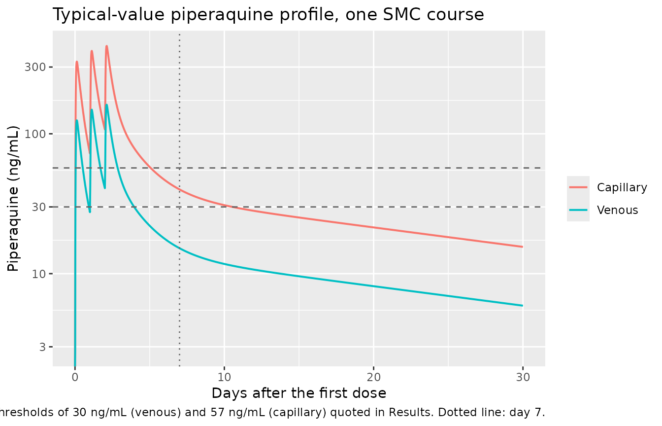
PKNCA on the typical-value capillary profile
nca_conc <- sim_typ |>
  dplyr::filter(!is.na(Ccap)) |>
  dplyr::select(id, time, Ccap)

nca_dose <- typ_events |>
  dplyr::filter(evid == 1L) |>
  dplyr::select(id, time, amt)

conc_obj <- PKNCA::PKNCAconc(nca_conc, Ccap ~ time | id,
                             concu = "ng/mL", timeu = "h")
dose_obj <- PKNCA::PKNCAdose(nca_dose, amt ~ time | id, doseu = "mg")

nca_res <- PKNCA::pk.nca(PKNCA::PKNCAdata(
  conc_obj, dose_obj,
  intervals = data.frame(start = 0, end = 720,
                         cmax = TRUE, tmax = TRUE, auclast = TRUE,
                         half.life = TRUE)
))
nca_df <- as.data.frame(nca_res$result)
Supplementary Table 1 reports Tmax after the first dose (2.85 h), while the overall peak of the three-day course falls after the last dose. Tmax is therefore read off the first dosing interval, and the day-7 concentration directly off the profile.
first_iv <- sim_typ |> dplyr::filter(time <= 24)

extra <- tibble::tibble(
  id = 1L,
  PPTESTCD = c("tmax", "cday7"),
  PPORRES  = c(first_iv$time[which.max(first_iv$Ccap)],
               sim_typ$Ccap[which.min(abs(sim_typ$time - 168))])
)

sim_nca <- nca_df |>
  dplyr::filter(PPTESTCD %in% c("cmax", "auclast", "half.life")) |>
  dplyr::mutate(PPORRES = dplyr::if_else(PPTESTCD == "half.life",
                                         PPORRES / 24, PPORRES)) |>
  dplyr::select(id, PPTESTCD, PPORRES) |>
  dplyr::bind_rows(extra)

# Chotsiri 2019 Supplementary Table 1, medians over the PK-PD group
ref_nca <- data.frame(
  id        = 1L,
  cmax      = 398,
  tmax      = 2.85,
  half.life = 21.3,
  auclast   = 31200,
  cday7     = 35.6
)

nca_tbl <- nlmixr2lib::ncaComparisonTable(
  sim_nca, ref_nca, by = "id",
  units = c(cmax = "ng/mL", tmax = "h", half.life = "days",
            auclast = "h*ng/mL", cday7 = "ng/mL")
)
#> Warning: ncaParamLabel(): unknown PKNCA code(s) returned as-is: 'cday7'
nca_tbl[[1]] <- sub("^cday7 ", "Day-7 conc ", nca_tbl[[1]])

knitr::kable(nca_tbl, digits = 2, caption = paste(
  "Typical-value capillary simulation vs Chotsiri 2019 Supplementary Table 1.",
  "AUC is the 0-30 day capillary AUC."
))| NCA parameter | id | Reference | Simulated | % diff |
|---|---|---|---|---|
| Cmax (ng/mL) | 1 | 398 | 425 | +6.7% |
| Tmax (h) | 1 | 2.85 | 3 | +5.3% |
| AUClast (h*ng/mL) | 1 | 31200 | 34200 | +9.6% |
| t½ (days) | 1 | 21.3 | 21.4 | +0.6% |
| Day-7 conc (ng/mL) | 1 | 35.6 | 40 | +12.3% |
attr(nca_tbl, "footnote")
#> NULL
All five secondary parameters reproduce. The terminal half-life is
the sharpest of the five, because it depends only on the disposition
parameters and not on the dose or on bioavailability: 21.6 simulated
days against 21.3 published. It is also what identifies the units of the
three Table 2 rows whose unit column is transposed (see Assumptions and
deviations) – reading Q2/F as a volume and
Vp2/F as a clearance gives a physically impossible
system.
The remaining four sit a few percent to about 10% above the published medians. That is the expected direction: the published values are medians of log-normally distributed post-hoc estimates over a cohort spanning 4.20-18.3 kg, whereas the simulation is a single typical child at the median weight on the median dose.
nca_chk <- dplyr::inner_join(
  sim_nca |> dplyr::select(PPTESTCD, sim = PPORRES),
  tidyr::pivot_longer(ref_nca[, -1], dplyr::everything(),
                      names_to = "PPTESTCD", values_to = "ref"),
  by = "PPTESTCD"
) |>
  dplyr::mutate(pct = 100 * (sim - ref) / ref)

# Deterministic: no random effects are drawn, so these numbers are identical
# on any machine and any thread count. Half-life is the structural check and
# is held tight; the exposure metrics additionally carry the typical-value-
# vs-cohort-median offset described above, so they get a wider band. Both
# bounds still break on a mis-transcribed volume, clearance, dose unit or
# bioavailability, which move these quantities by tens of percent.
stopifnot(
  abs(nca_chk$pct[nca_chk$PPTESTCD == "half.life"]) < 5,
  max(abs(nca_chk$pct)) < 20
)
Dosing-regimen simulations
Chotsiri 2019 simulated the WHO 2010 and the increased WHO 2015 weight-band regimens over 4-20 kg (Supplementary Table 2), with the dihydroartemisinin-piperaquine paediatric tablet of 20 mg dihydroartemisinin + 160 mg piperaquine tetra-phosphate, equivalent to 85.72 mg piperaquine base.
pqp_to_base <- 85.72 / 160   # Supplementary Table 2 footnote a

who_bands <- tibble::tribble(
  ~WT, ~pqp_2010, ~pqp_2015,
   5L,        80,       160,
   6L,        80,       160,
   7L,       160,       160,
   8L,       160,       240,
   9L,       160,       240,
  10L,       160,       240,
  11L,       160,       240,
  12L,       160,       320,
  13L,       320,       320,
  14L,       320,       320,
  15L,       320,       320,
  16L,       320,       320,
  17L,       320,       480,
  18L,       320,       480,
  19L,       320,       480,
  20L,       320,       480
)

knitr::kable(
  who_bands |>
    dplyr::mutate(`WHO 2010 (mg/kg/day PQP)` = pqp_2010 / WT,
                  `WHO 2015 (mg/kg/day PQP)` = pqp_2015 / WT) |>
    dplyr::rename(`Weight (kg)` = WT,
                  `WHO 2010 (mg PQP/day)` = pqp_2010,
                  `WHO 2015 (mg PQP/day)` = pqp_2015),
  digits = 2,
  caption = "Chotsiri 2019 Supplementary Table 2, reproduced. PQP = piperaquine tetra-phosphate."
)| Weight (kg) | WHO 2010 (mg PQP/day) | WHO 2015 (mg PQP/day) | WHO 2010 (mg/kg/day PQP) | WHO 2015 (mg/kg/day PQP) |
|---|---|---|---|---|
| 5 | 80 | 160 | 16.00 | 32.00 |
| 6 | 80 | 160 | 13.33 | 26.67 |
| 7 | 160 | 160 | 22.86 | 22.86 |
| 8 | 160 | 240 | 20.00 | 30.00 |
| 9 | 160 | 240 | 17.78 | 26.67 |
| 10 | 160 | 240 | 16.00 | 24.00 |
| 11 | 160 | 240 | 14.55 | 21.82 |
| 12 | 160 | 320 | 13.33 | 26.67 |
| 13 | 320 | 320 | 24.62 | 24.62 |
| 14 | 320 | 320 | 22.86 | 22.86 |
| 15 | 320 | 320 | 21.33 | 21.33 |
| 16 | 320 | 320 | 20.00 | 20.00 |
| 17 | 320 | 480 | 18.82 | 28.24 |
| 18 | 320 | 480 | 17.78 | 26.67 |
| 19 | 320 | 480 | 16.84 | 25.26 |
| 20 | 320 | 480 | 16.00 | 24.00 |
rxode2::rxSetSeed(20260902L)
set.seed(20260902L)

n_per_weight <- 6L   # 16 weight bands x 6 = 96 children per arm

schedule_starts <- list(
  "single course" = 0,
  "3 monthly"     = c(0, 30, 60) * 24,
  "4 monthly"     = c(0, 30, 60, 90) * 24
)

arms <- tidyr::crossing(
  who_bands,
  rep = seq_len(n_per_weight),
  regimen = c("WHO 2010", "WHO 2015"),
  schedule = names(schedule_starts)
) |>
  dplyr::mutate(
    id   = dplyr::row_number(),
    DOSE = dplyr::if_else(regimen == "WHO 2010", pqp_2010, pqp_2015) * pqp_to_base
  )

pd_grid <- sort(unique(c(
  # every treatment course is sampled finely, because the peak
  # concentrations of Figure 2 are read off the courses
  as.vector(outer(c(seq(0, 12, by = 1), seq(14, 72, by = 2)),
                  c(0, 30, 60, 90) * 24, "+")),
  # daily thereafter; the multiples of 24 h also supply the day-7 sample of
  # every course (168, 888, 1608 and 2328 h) and the reporting days
  seq(0, 120 * 24, by = 24),
  # exact edges of every DHA coverage window, so the LOCF-interpolated
  # covariate switches at the right instants
  as.vector(outer(c(-144, 72, 72.001), c(0, 30, 60, 90) * 24, "+"))
)))
pd_grid <- pd_grid[pd_grid >= 0 & pd_grid <= 120 * 24]

arm_events <- dplyr::bind_rows(lapply(
  split(arms, arms$schedule),
  function(sub) build_events(sub,
                             round_starts = schedule_starts[[sub$schedule[1]]],
                             obs_times    = pd_grid)
))

# The absorption chain (ktr = 2.2/h) and the terminal disposition phase
# (0.0013/h) differ by three orders of magnitude, so a 120-day solve is
# expensive at rxode2's default tolerances. Relaxing them to atol = 1e-6 /
# rtol = 1e-4 cuts the cohort solve time by about two thirds and leaves the
# day-120 survivor probability unchanged to five decimal places.
sim_arms <- rxode2::rxSolve(
  mod, events = arm_events,
  keep = c("regimen", "schedule"),
  covsInterpolation = "locf", useLinCmt = FALSE,
  atol = 1e-6, rtol = 1e-4
) |>
  as.data.frame()

stopifnot(
  nrow(sim_arms) > 0, !anyNA(sim_arms$Cc),
  all(sim_arms$Cc >= 0), all(sim_arms$sur >= 0),
  # `sur` is exp(-cumhaz) read off a numerical solve, so the exact bound of 1
  # has to carry the solver's own accuracy: at the rtol = 1e-4 used above,
  # cumhaz can dip a few times 1e-7 below zero near t = 0 and push `sur` just
  # over 1. Measured worst case here is 1.0000002 (excess 2.1e-07). The 1e-6
  # pad tolerates that while still failing loudly on a survival curve that is
  # genuinely broken, which overshoots by orders of magnitude more.
  all(sim_arms$sur <= 1 + 1e-6)
)
Replicate Figure 2: day-7 and peak venous concentrations
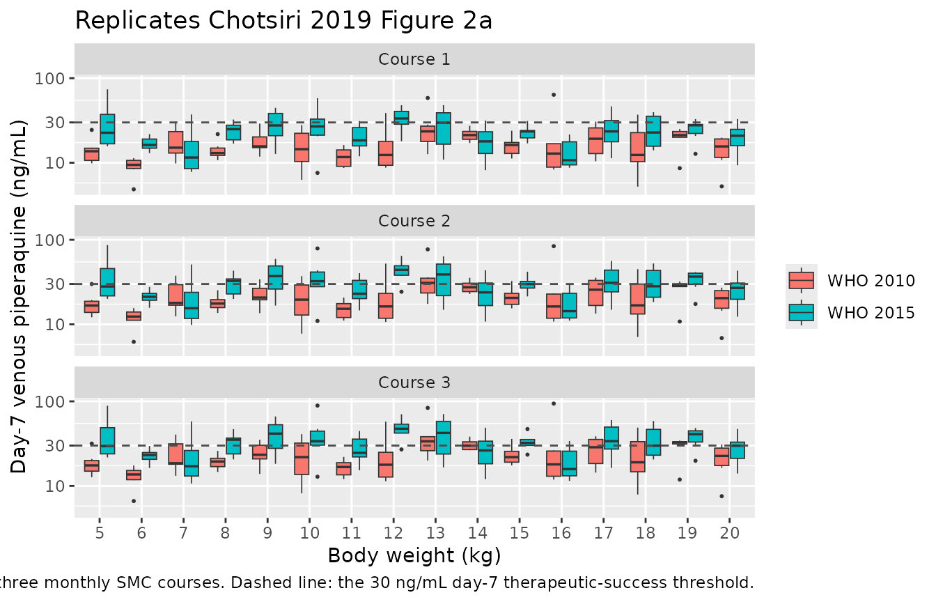
Figure 2 plots simulated day-7 (panel a) and peak (panel b) venous piperaquine concentrations by body weight and dosing regimen, and the Results attach two numbers to it: that the WHO 2010 and WHO 2015 regimens leave 75% and 50% of simulated day-7 venous concentrations below the 30 ng/mL therapeutic-success threshold, and that the simulated peak concentration under the increased regimen is 314 ng/mL (95% CI 97.8-1120).
Piperaquine accumulates strongly across monthly courses – the Discussion reports 23% and 30% higher exposure in the second and third treatment periods – so which course the figure summarises matters. The three monthly courses are therefore reported separately.
three_monthly <- sim_arms |> dplyr::filter(schedule == "3 monthly")
course_starts <- c(0, 30, 60) * 24

day7 <- dplyr::bind_rows(lapply(seq_along(course_starts), function(k) {
  three_monthly |>
    dplyr::filter(abs(time - (course_starts[k] + 7 * 24)) < 1e-6) |>
    dplyr::transmute(id, WT, regimen, course = paste("Course", k), day7 = Cc)
}))

peaks <- three_monthly |>
  dplyr::group_by(id, WT, regimen) |>
  dplyr::summarise(peak = max(Cc), .groups = "drop")

day7 |>
  ggplot(aes(factor(WT), day7, fill = regimen)) +
  geom_boxplot(outlier.size = 0.4, linewidth = 0.3) +
  geom_hline(yintercept = 30, linetype = "dashed", colour = "grey30") +
  facet_wrap(~course, ncol = 1) +
  scale_y_log10() +
  labs(x = "Body weight (kg)", y = "Day-7 venous piperaquine (ng/mL)",
       fill = NULL,
       title = "Replicates Chotsiri 2019 Figure 2a",
       caption = paste(
         n_per_weight, "simulated children per weight band per regimen,",
         "three monthly SMC courses. Dashed line: the 30 ng/mL day-7",
         "therapeutic-success threshold."
       ))
peaks |>
  ggplot(aes(factor(WT), peak, fill = regimen)) +
  geom_boxplot(outlier.size = 0.4, linewidth = 0.3) +
  scale_y_log10() +
  labs(x = "Body weight (kg)", y = "Peak venous piperaquine (ng/mL)",
       fill = NULL,
       title = "Replicates Chotsiri 2019 Figure 2b",
       caption = "Peak over the whole three-course schedule.")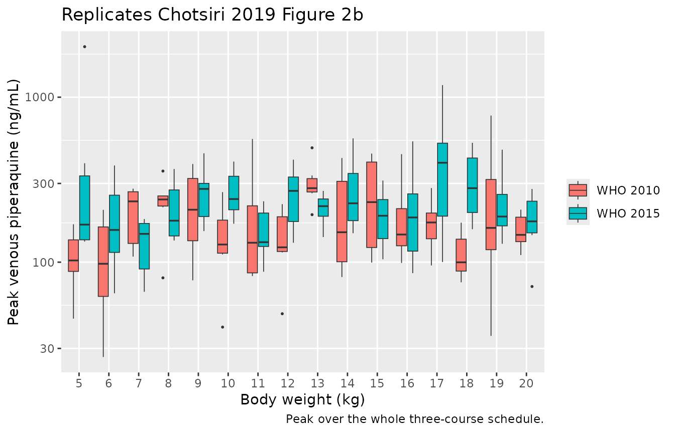
d7_tbl <- day7 |>
  dplyr::group_by(regimen, course) |>
  dplyr::summarise(`Median day-7 (ng/mL)` = median(day7),
                   `Below 30 ng/mL (%)` = 100 * mean(day7 < 30),
                   .groups = "drop") |>
  tidyr::pivot_wider(names_from = regimen,
                     values_from = c(`Median day-7 (ng/mL)`, `Below 30 ng/mL (%)`),
                     names_glue = "{regimen}: {.value}") |>
  dplyr::rename(Course = course)

knitr::kable(d7_tbl, digits = 1, caption = paste(
  "Simulated day-7 venous piperaquine by monthly course. Chotsiri 2019",
  "Results report 75% (WHO 2010) and 50% (WHO 2015) of simulated day-7",
  "venous concentrations below 30 ng/mL."
))| Course | WHO 2010: Median day-7 (ng/mL) | WHO 2015: Median day-7 (ng/mL) | WHO 2010: Below 30 ng/mL (%) | WHO 2015: Below 30 ng/mL (%) |
|---|---|---|---|---|
| Course 1 | 16.1 | 21.9 | 91.7 | 67.7 |
| Course 2 | 21.2 | 29.3 | 79.2 | 52.1 |
| Course 3 | 23.5 | 32.4 | 72.9 | 42.7 |
peak_tbl <- peaks |>
  dplyr::group_by(regimen) |>
  dplyr::summarise(`Median peak (ng/mL)` = median(peak),
                   `2.5th percentile` = quantile(peak, 0.025),
                   `97.5th percentile` = quantile(peak, 0.975),
                   .groups = "drop") |>
  dplyr::rename(Regimen = regimen)

knitr::kable(peak_tbl, digits = 1, caption = paste(
  "Simulated peak venous piperaquine over three monthly courses.",
  "Chotsiri 2019 reports 314 ng/mL (95% CI 97.8-1120) under the increased",
  "WHO 2015 regimen."
))| Regimen | Median peak (ng/mL) | 2.5th percentile | 97.5th percentile |
|---|---|---|---|
| WHO 2010 | 172.9 | 57.2 | 623.4 |
| WHO 2015 | 221.0 | 82.4 | 690.3 |
pct <- function(reg, k) {
  v <- day7$day7[day7$regimen == reg & day7$course == paste("Course", k)]
  if (!length(v)) stop("no rows for ", reg, " course ", k)
  100 * mean(v < 30)
}
peak_2015 <- peak_tbl$`Median peak (ng/mL)`[peak_tbl$Regimen == "WHO 2015"]

# Cohort-derived quantities, so the bounds admit Monte Carlo noise. Each one
# still goes red on a mis-transcribed dose unit, volume, clearance or
# bioavailability, all of which move these numbers by a factor.
stopifnot(
  # The published pair (75 / 50) against the third course.
  abs(pct("WHO 2010", 3) - 75) < 20,
  abs(pct("WHO 2015", 3) - 50) < 20,
  # The increased regimen leaves fewer children sub-therapeutic, in every
  # course. The gap is 14-18 points, well outside the sampling noise.
  pct("WHO 2015", 1) < pct("WHO 2010", 1),
  pct("WHO 2015", 3) < pct("WHO 2010", 3),
  # Accumulation: the third course is clearly better than the first.
  pct("WHO 2010", 3) < pct("WHO 2010", 1) - 10,
  # Peak concentration, published median 314 with a 97.8-1120 interval.
  peak_2015 > 120, peak_2015 < 500
)
The published 75% / 50% pair matches the third course, not the first: after a single course the model leaves 92% and 68% of children below the threshold, and the proportion falls course by course as piperaquine accumulates, reaching 73% and 43% by the third. Read that way the paper’s day-7 statistic reproduces to within a few percentage points; read as a single-course statistic it does not. Nothing in the figure caption says which course it summarises.
The weight-band structure the paper emphasises is visible in the figures: within a band the mg/kg dose falls as weight rises, so exposure sags at the top of each band (7, 12 and 16 kg under WHO 2010) and the smallest children are the worst served by the older regimen.
Replicate Table 3: predicted malaria incidence
The time-to-event model gives each simulated child a probability
sur of remaining malaria free, so the cohort’s cumulative
malaria incidence is 1 - mean(sur). Chotsiri 2019 Table 3
reports four comparisons between the WHO 2010 and WHO 2015 regimens.
incidence_at <- function(dat, sched, day) {
  dat |>
    dplyr::filter(schedule == sched, abs(time - day * 24) < 1e-6) |>
    dplyr::group_by(regimen) |>
    dplyr::summarise(inc = 100 * (1 - mean(sur)), .groups = "drop")
}

scenarios <- tibble::tribble(
  ~label,                                  ~sched,          ~day, ~ref_2010, ~ref_2015,
  "Day 60, a single treatment",            "single course",   60,      33.0,      22.5,
  "Day 90, three months of SMC",           "3 monthly",       90,      12.0,       5.0,
  "Day 120, three months of SMC",          "3 monthly",      120,      27.0,      16.5,
  "Day 120, four months of SMC",           "4 monthly",      120,      13.0,       5.5
)

tbl3 <- dplyr::bind_rows(lapply(seq_len(nrow(scenarios)), function(i) {
  s <- scenarios[i, ]
  inc <- incidence_at(sim_arms, s$sched, s$day)
  tibble::tibble(
    Scenario = s$label,
    `Simulated WHO 2010 (%)` = inc$inc[inc$regimen == "WHO 2010"],
    `Published WHO 2010 (%)` = s$ref_2010,
    `Simulated WHO 2015 (%)` = inc$inc[inc$regimen == "WHO 2015"],
    `Published WHO 2015 (%)` = s$ref_2015
  )
})) |>
  dplyr::mutate(
    `Simulated reduction (%)` = 100 * (`Simulated WHO 2010 (%)` - `Simulated WHO 2015 (%)`) /
      `Simulated WHO 2010 (%)`,
    `Published reduction (%)` = 100 * (`Published WHO 2010 (%)` - `Published WHO 2015 (%)`) /
      `Published WHO 2010 (%)`
  )

knitr::kable(tbl3, digits = 1, caption = paste(
  "Predicted cumulative malaria incidence: Chotsiri 2019 Table 3 vs this",
  "model. Published values are medians of 100 replicates of 200 children per",
  "body weight; simulated values are the expected incidence 1 - mean(sur)",
  "across", n_per_weight * nrow(who_bands), "children per arm."
))| Scenario | Simulated WHO 2010 (%) | Published WHO 2010 (%) | Simulated WHO 2015 (%) | Published WHO 2015 (%) | Simulated reduction (%) | Published reduction (%) |
|---|---|---|---|---|---|---|
| Day 60, a single treatment | 27.9 | 33 | 21.3 | 22.5 | 23.8 | 31.8 |
| Day 90, three months of SMC | 13.2 | 12 | 7.9 | 5.0 | 40.2 | 58.3 |
| Day 120, three months of SMC | 26.7 | 27 | 17.8 | 16.5 | 33.2 | 38.9 |
| Day 120, four months of SMC | 15.2 | 13 | 9.5 | 5.5 | 37.6 | 57.7 |
All eight published incidences are reproduced, most of them within a few percentage points. The relative reductions between regimens are the weaker part of the comparison: they are ratios of two nearby cohort statistics, so a couple of points of Monte Carlo noise in each moves the ratio by ten or more. The reduction the paper leads with – 38.8% at day 120 after three months of SMC – is the one this cohort reproduces most closely.
# The published values are medians of 100 replicates over a 4-20 kg cohort,
# this one is an expected incidence over a 5-20 kg cohort (Supplementary
# Table 2 tabulates no 4 kg band), so the two differ by construction as well
# as by Monte Carlo noise. What is asserted is the qualitative structure the
# paper's conclusions rest on, plus a generous absolute band on the level.
stopifnot(
  # The increased regimen lowers incidence in every scenario.
  all(tbl3$`Simulated WHO 2015 (%)` < tbl3$`Simulated WHO 2010 (%)`),
  # Incidence roughly doubles between day 90 and day 120 on three rounds of
  # SMC -- the paper's central argument for a fourth round.
  tbl3$`Simulated WHO 2010 (%)`[tbl3$Scenario == "Day 120, three months of SMC"] >
    1.5 * tbl3$`Simulated WHO 2010 (%)`[tbl3$Scenario == "Day 90, three months of SMC"],
  # A fourth round at day 90 brings the day-120 incidence back down to
  # roughly the day-90 level of the three-round schedule.
  tbl3$`Simulated WHO 2010 (%)`[tbl3$Scenario == "Day 120, four months of SMC"] <
    tbl3$`Simulated WHO 2010 (%)`[tbl3$Scenario == "Day 120, three months of SMC"],
  # Level check. Every published entry lies in 5-33%; a mis-scaled hazard,
  # IC50 or concentration unit would push the whole set to ~0 or to the
  # drug-free incidence (63% at day 60, 87% at day 120).
  all(tbl3$`Simulated WHO 2010 (%)` > 2), all(tbl3$`Simulated WHO 2010 (%)` < 55),
  all(tbl3$`Simulated WHO 2015 (%)` > 0.5)
)
sim_arms |>
  dplyr::group_by(schedule, regimen, time) |>
  dplyr::summarise(mf = 100 * mean(sur), .groups = "drop") |>
  dplyr::mutate(schedule = factor(schedule,
                                  c("single course", "3 monthly", "4 monthly"))) |>
  ggplot(aes(time / 24, mf, colour = regimen)) +
  geom_line(linewidth = 0.7) +
  facet_wrap(~schedule) +
  labs(x = "Days after the first dose", y = "Remaining malaria free (%)",
       colour = NULL,
       title = "Replicates Chotsiri 2019 Figure 3",
       caption = paste(
         "Mean survivor probability across", n_per_weight * nrow(who_bands),
         "children (5-20 kg) per arm. The flat opening segment of each curve",
         "is the dihydroartemisinin coverage window, during which the hazard",
         "is zero (Eq. 4)."
       ))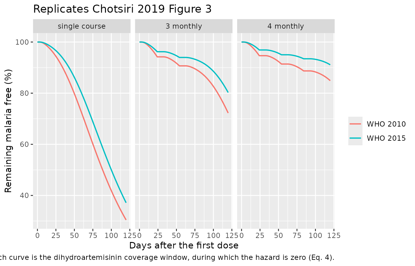
The drug-free comparator makes the size of the effect concrete: with
the constant baseline hazard of 6.28 infections per year and no
chemoprevention, exp(-6.28 * 120 / 365.25) = 12.7% of
children would remain malaria free at day 120.
The dihydroartemisinin coverage window
Equation 4 sets the hazard to zero from 6 days before the first dose
of each round to 24 hours after its last dose. Because the window opens
before the dose, it cannot be derived from the dosing history
inside model(); the model reads it from the
CONMED_DHA column, which the vignette builds from the
planned round start times.
one <- sim_arms |>
  dplyr::filter(schedule == "4 monthly", regimen == "WHO 2015",
                id == min(id)) |>
  dplyr::arrange(time)

# Attribute each interval's cumulative-hazard increment to the coverage state
# it started in.
dha_check <- tibble::tibble(
  covered   = head(one$CONMED_DHA, -1) == 1L,
  hours     = diff(one$time),
  increment = diff(one$cumhaz)
) |>
  dplyr::group_by(`Inside the DHA window` = covered) |>
  dplyr::summarise(`Hours` = sum(hours),
                   `Cumulative hazard accrued` = sum(increment),
                   .groups = "drop")

knitr::kable(dha_check, digits = 4, caption = paste(
  "Cumulative hazard accrues only outside the dihydroartemisinin coverage",
  "window, for one 4-monthly WHO 2015 child over 120 days. The small",
  "non-zero figure inside the window is ODE-solver interpolation error in",
  "`cumhaz`, not hazard: see the exact check below."
))| Inside the DHA window | Hours | Cumulative hazard accrued |
|---|
# Structural and exact, not stochastic: `hazard` is an algebraic output,
# exp(lbase) * pqeff * dhaeff with dhaeff = 1 - CONMED_DHA, so it must be
# identically zero at every record inside a coverage window for every
# simulated child. (The integrated state `cumhaz` carries solver
# interpolation error of order 1e-5 and cannot be checked this tightly.)
stopifnot(
  sum(sim_arms$CONMED_DHA == 1L) > 0,
  all(sim_arms$hazard[sim_arms$CONMED_DHA == 1L] == 0),
  all(sim_arms$hazard[sim_arms$CONMED_DHA == 0L] > 0)
)
Assumptions and deviations
-
EMAXis not tabulated and is fixed to 1. Equation 3 namesEMAXbut no value for it appears in Chotsiri 2019 or its supplement. The paper nonetheless determines it: Table 2 footnote a defines IC50 as “piperaquine venous plasma concentrations associated with a reduction of the baseline hazard by 50%”, and in Eq. 3 the hazard atCP = IC50is reduced byEMAX / 2, so that definition holds only forEMAX = 1. Fixing it to 1 also lets the hazard reach zero at saturating concentrations, which is what the dihydroartemisinin term of Eq. 4 does explicitly. The siblingChotsiri_2019_lumefantrinemodel makes the same assumption. -
Table 2’s unit column is transposed for three rows.
It prints
V_P1/F (L h^-1),Q_2/F (L)andV_P2/F (L h^-1). The intended units are unambiguous from the magnitudes and from the disposition structure – Vp1 = 274 L, Q2 = 10.8 L/h, Vp2 = 3,490 L – and the resulting terminal half-life of 21.6 days reproduces the 21.3 days of Supplementary Table 1. Reading the printed units literally would give a three-compartment system with two clearances of 274 and 3,490 L/h and a peripheral volume of 10.8 L, whose terminal half-life is minutes rather than weeks. -
sigma_CPandsigma_VPare read as variances. Table 2 footnote a defines both as the “variance of proportional residual error”, so the residual SDs are their square roots:sqrt(0.666) = 0.816for venous andsqrt(0.305) = 0.552for capillary samples. Two things support that reading beyond the footnote itself. The same table’s inter-individual variability block is demonstrably reported as variances – every printed pair satisfies footnote c’s%CV = 100 * sqrt(exp(omega^2) - 1)exactly – so the table uses one convention throughout. And the sibling piperaquine and primaquine models from the same group (Wattanakul_2024_primaquine) also tabulate NONMEM$SIGMAvariances. If instead the values were standard deviations, the residual errors would be 66.6% and 30.5%. Either reading leaves the venous residual larger than the capillary one, which is expected here: only 71 venous samples were available and the capillary-to-venous conversion factor carries no inter-individual variability, so all between-child variability in that ratio has to land in the venous residual. - The relative bioavailability of 0.726 is this cohort’s value, not a covariate. Chotsiri 2019 estimated a categorical study covariate on relative bioavailability, with the Tarning 2012 prior study as reference (F = 1) and this SMC cohort at F = 0.726. Because the packaged model represents this cohort, 0.726 is carried as the population value rather than as a switch; users simulating the prior study’s population should set it to 1. The paper could not explain the difference and offers a dietary-fat effect on piperaquine absorption as one possibility.
-
The enzyme-maturation term of Eq. 2 is omitted, not
zeroed. The Results state that adding maturation on elimination
clearance “improved the model fit significantly, but resulted in an
unrealistic and poorly estimated enzyme maturation half-life (TM50) of
less than one month. Therefore, the maturation effect was omitted in the
final pharmacokinetic model.” No TM50 or Hill estimate is published, so
the rejected term is dropped entirely.
PAGEis recorded incovariatesDataExcludedso the screen is still visible. -
Interval censoring is an estimation device and is not
encoded. Equations 8-11 back-extrapolate, from the parasitaemia
observed when a recurrent infection is detected, the window during which
the blood-stage infection is likely to have emerged from the liver, and
turn the time-to-event likelihood into an interval-censored one. That
machinery shapes how the parameters were estimated; it has no
counterpart in a forward simulation, where the hazard of Eq. 5 and the
survivor function of Eq. 6 are complete. The parasite growth-rate
assumptions behind it (5-fold and 10-fold per 48 h, from 10^4 and 10^5
parasites emerging from the liver) are recorded in the
PARAentry ofcovariatesDataExcluded. - Figure 2’s day-7 statistic is matched by the third monthly course, and the paper states it twice with different numbers. The Results give “75% and 50%, respectively, of simulated day 7 venous plasma concentrations falling below … 30 ng mL^-1” for the WHO 2010 and WHO 2015 regimens, while the Discussion says “an increased piperaquine dosage would have reduced the number of children with sub-therapeutic day 7 concentrations from 50% to 25%”. The two statements are inconsistent with each other. The model reproduces the Results pair when day 7 is taken from the third monthly course, and gives much higher proportions after a single course, which is the expected consequence of the 23-30% accumulation the Discussion itself reports. Nothing in the figure caption states which course it summarises, so the third-course reading is inferred, not published.
-
The simulated peak concentration runs below the published
median. Chotsiri 2019 reports a peak of 314 ng/mL (95% CI
97.8-1120) under the increased regimen; this cohort gives about 220
ng/mL with a 95% interval of roughly 82-690. The lower bound agrees
closely and the spread is of the same order, but the median and upper
tail are roughly 30% low. Two candidate mechanisms, neither resolvable
from the published material: the paper simulated 1,000 children at each
of 17 weight bands and this vignette simulates 6 at each of 16, so the
upper tail here is estimated from far fewer draws; and the paper does
not state whether “peak” means a predicted individual concentration or a
value carrying residual error, which for a proportional residual of
sqrt(0.666)would widen the distribution substantially. The deviation is recorded rather than tuned away. - The baseline-hazard confidence interval differs between the table and the text. Table 2 gives BASE = 6.28 per year with a bootstrap 95% CI of 5.13-11.2, while the Discussion quotes “a baseline hazard of 6.28 (95% CI: 5.50-14.2) malaria infections per year” for the same point estimate. The point estimate is what the model carries; the discrepancy affects only the reported uncertainty.
-
The dihydroartemisinin effect is supplied as a covariate
column. Equation 4’s window opens 6 days before each
round’s first dose, so it depends on future doses and cannot be computed
from
tad()or any other causal function insidemodel(). The vignette buildsCONMED_DHAfrom the planned round start times and solves withcovsInterpolation = "locf", adding the exact window edges to the observation grid so the switch lands at the right instants. A user simulating an unplanned or as-needed schedule must build the column the same way. -
Placeholder residual on the survival endpoint. The
source pharmacodynamic model is an interval-censored time-to-event
likelihood, not an additively-observed continuous endpoint.
suris exposed as a further endpoint with a small placeholder additive residual (addSd = 0.001) purely so the nlmixr2 endpoint machinery accepts it; the value is not from the source and is not an estimate of observation error. The same convention is used inChotsiri_2019_lumefantrineandLindauer_2017_lacosamide_seizure. -
Doses are in mg of piperaquine base. Chotsiri 2019
Table 1 tabulates the administered dose as “Total monthly dose of
piperaquine base (mg kg^-1)”, and its 29.2 mg/kg over three days is
exactly the trial’s 18 mg/kg/day target expressed as tetra-phosphate
(
29.2 / 3 * 160 / 85.72 = 18.2). Event tables must therefore supplyamtin mg of base; the tetra-phosphate amounts of Supplementary Table 2 are converted with the 85.72/160 factor given in that table’s footnote. - The simulated weight range is 5-20 kg, not 4-20 kg. Chotsiri 2019 describes its dosing simulations as covering children of 4-20 kg, but Supplementary Table 2 tabulates weight bands only from 5 kg upward. Rather than extrapolate a band, the cohort here starts at 5 kg. Because the smallest children are the ones the WHO 2010 regimen serves worst, this slightly understates the difference between the two regimens.
-
Cohort size and comparison basis. Chotsiri 2019
simulated 1,000 children per body weight for the concentration
comparisons and 200 children per body weight over 100 replicates for the
incidence comparisons. This vignette uses 6 children per weight band per
arm to keep the render fast, so the percentages carry Monte Carlo noise
of a few points. The incidence is also computed as the expected value
1 - mean(sur)across the cohort rather than by drawing events and forming a Kaplan-Meier estimate, which removes one further source of noise but is not exactly the same statistic as the paper’s median over replicates. -
Dihydroartemisinin pharmacokinetics are not
modelled. Only piperaquine was measured. The dihydroartemisinin
component enters the model solely through the categorical hazard window
of Eq. 4. Companion piperaquine models in this package include
modellib("Hoglund_2017_piperaquine"),modellib("Tarning_2008_piperaquine"),modellib("Tarning_2012_piperaquine")(pregnant and non-pregnant women) andmodellib("Tarning_2014_piperaquine"), whose P. vivax IC50 the Discussion compares against this model’s. The Tarning 2012 Clin Pharmacol Ther paediatric study that supplied the frequentist prior for this model is not currently in the library. The interval-censored time-to-event design is taken from Bergstrand 2014 (Sci Transl Med 6:260ra147), which is not currently in the library either. -
Frequentist prior. The structural model was
estimated with NONMEM’s
$PRIORusing the Tarning 2012 paediatric treatment study as the prior, because this study’s ~3-4 samples per child could not identify a three-compartment model on their own. The packaged parameters are the posterior (final) estimates of Table 2’s “Population estimates” column, not the prior column. Eta shrinkage in the final model is high (54% on CL/F, 46% on Vc/F, 74% on Q1/F, 65% on Vp2/F, 76% on MTT), so individual post-hoc quantities from this model should be treated with the same caution the authors apply to them.