Hyaluronic acid dermal filler residence in hairless mice (Ryu 2021)
Source:vignettes/articles/Ryu_2021_hyaluronicAcid_fillers_mouse.Rmd
Ryu_2021_hyaluronicAcid_fillers_mouse.RmdModel and source
Ryu 2021 fitted one swelling-degradation kinetic model separately to each of five marketed hyaluronic acid (HA) dermal fillers. The five fits share a structure but no parameters, so they are extracted as five model files that share this vignette.
fillers <- tibble::tribble(
  ~filler, ~model, ~gel_phase,
  "99 fill", "Ryu_2021_hyaluronicAcid_99fill_mouse", "mono-phasic",
  "Juvederm VOLUMA with Lidocaine", "Ryu_2021_hyaluronicAcid_juvedermVoluma_mouse", "mono-phasic",
  "Neuramis VOLUME Lidocaine", "Ryu_2021_hyaluronicAcid_neuramisVolume_mouse", "mono-phasic",
  "Restylane Lyft with Lidocaine", "Ryu_2021_hyaluronicAcid_restylaneLyft_mouse", "bi-phasic",
  "YVOIRE Contour plus", "Ryu_2021_hyaluronicAcid_yvoireContourPlus_mouse", "bi-phasic"
)
fillers$filler <- factor(fillers$filler, levels = fillers$filler)
uis <- lapply(fillers$model, function(m) rxode2::rxode(readModelDb(m)))
#> ℹ parameter labels from comments will be replaced by 'label()'
#> ℹ parameter labels from comments will be replaced by 'label()'
#> ℹ parameter labels from comments will be replaced by 'label()'
#> ℹ parameter labels from comments will be replaced by 'label()'
#> ℹ parameter labels from comments will be replaced by 'label()'
names(uis) <- as.character(fillers$filler)- Article: https://doi.org/10.3390/pharmaceutics13020133
- Supplement (Table S1 filler properties, Text S1 NONMEM control stream, Figure S1 goodness of fit): https://www.mdpi.com/1999-4923/13/2/133/s1
- Citation: Ryu H-j, Kwak S-s, Rhee C-h, Yang G-h, Yun H-y, Kang W-h. Model-Based Prediction to Evaluate Residence Time of Hyaluronic Acid Based Dermal Fillers. Pharmaceutics. 2021;13(2):133. doi:10.3390/pharmaceutics13020133. Parameter estimates from Table 1; structure from Equations 1-4 and Supplementary Text S1 (the NONMEM 7.4 control stream deposited for Neuramis VOLUME Lidocaine; the same structure was fitted to each filler).
Description of the Neuramis model (the other four differ only in the filler named and, for 99 fill, a slope fixed to zero): Preclinical (mouse). Swelling-degradation kinetic model of the residual volume of the hyaluronic acid dermal filler Neuramis VOLUME Lidocaine (Medytox; mono-phasic, BDDE-cross-linked, 1.0 x 10^6 Da HA, 20 mg/mL) after a single 100 uL subcutaneous injection into the dorsal skin of hairless mice (Ryu 2021). A depot compartment empties by first-order ‘swelling’ (Kswell) into a subcutaneous observation compartment that is lost by first-order ‘degradation’ (Kdeg); the observed filler volume is the subcutaneous amount. Between-animal variability is carried on Kswell only, and the Kdeg random effect is the Kswell random effect scaled by an estimated slope. One of five filler-specific fits from the same paper.
Population
Female SKH1-Hr hr hairless mice, six to seven weeks old at purchase, received a single 100 uL subcutaneous injection of one filler into the dorsal skin (n = 8 per filler; Methods 2.1). Filler volume under the skin was measured by 3D imaging (PRIMOS Lite) at 0, 1, 4, 7, 21 and 28 days and monthly from 2 to 18 months; the lower detection limit was 3 mm^3 (0.003 cm^3). All fillers are BDDE-cross-linked HA; their molecular weight, HA content and gel phase are in Supplementary Table S1 (99 fill properties are confidential), and the Discussion classifies 99 fill, Juvederm and Neuramis as mono-phasic and Restylane and YVOIRE as bi-phasic. No covariates were assessed.
The same information is available programmatically via each model’s
population metadata, e.g.
readModelDb("Ryu_2021_hyaluronicAcid_neuramisVolume_mouse")()$population.
Model structure
Equations 1-4 and Supplementary Text S1:
-
Kswell = theta1 * exp(eta1)andKdeg = theta2 * exp(theta3 * eta1)– a single random effect drives both rate constants, with the estimatedSlope(theta3,kdeg_eta_scalehere) scaling it ontoKdeg. -
d DEPOT / dt = -Kswell * DEPOTandd SC / dt = Kswell * DEPOT - Kdeg * SC, with the filler dosed intoDEPOT. - The observed volume is the subcutaneous amount
(
IPRED = A(2)) with a proportional residual error.
In the model files DEPOT is depot,
SC is central, Kswell is the
depot-to-observation first-order transfer and is carried as the
canonical absorption rate ka, and Kdeg is
kdeg. The observed filler volume is the
central state itself.
Source trace
Every value below is Table 1 of Ryu 2021 (the in-file comments give
the row for each). IIV is printed as a CV and converted with
omega^2 = log(1 + CV^2); the proportional residual CV is
used directly as propSd.
trace <- tibble::tribble(
  ~filler, ~Kswell_printed, ~Kdeg, ~Slope, ~IIV_Kswell_CV, ~prop_CV,
  "99 fill", 2.20, 1.45, "0 (fixed)", "17.9%", "16.3%",
  "Juvederm VOLUMA with Lidocaine", 3.04, 1.98, "1.15", "46.5%", "13.8%",
  "Neuramis VOLUME Lidocaine", 3.55, 2.20, "1.06", "22.3%", "14.9%",
  "Restylane Lyft with Lidocaine", 4.74, 4.24, "1.01", "29%", "17.9%",
  "YVOIRE Contour plus", 1.82, 1.47, "1.16", "25%", "11.2%"
)
# Each packaged model must carry exactly the Table 1 values (Kswell x 10^-3).
packaged <- bind_rows(lapply(names(uis), function(nm) {
  th <- uis[[nm]]$theta
  data.frame(
    filler = nm,
    ka = unname(exp(th["lka"])),
    kdeg = unname(exp(th["lkdeg"])),
    slope = unname(th["kdeg_eta_scale"]),
    omega = unname(uis[[nm]]$omega[1, 1]),
    propSd = unname(th["propSd"])
  )
}))
stopifnot(
  identical(packaged$filler, trace$filler),
  all(abs(packaged$ka / (trace$Kswell_printed * 1e-3) - 1) < 1e-12),
  all(abs(packaged$kdeg / trace$Kdeg - 1) < 1e-12),
  all(abs(packaged$slope - c(0, 1.15, 1.06, 1.01, 1.16)) < 1e-12),
  all(abs(packaged$omega - log(1 + c(0.179, 0.465, 0.223, 0.29, 0.25)^2)) < 1e-6),
  all(abs(packaged$propSd - c(0.163, 0.138, 0.149, 0.179, 0.112)) < 1e-12)
)
trace |>
  dplyr::rename(
    "Filler" = filler,
    "Kswell as printed (Table 1)" = Kswell_printed,
    "Kdeg (1/day)" = Kdeg,
    "Slope" = Slope,
    "IIV on Kswell (CV)" = IIV_Kswell_CV,
    "Proportional RV (CV)" = prop_CV
  ) |>
knitr::kable()| Filler | Kswell as printed (Table 1) | Kdeg (1/day) | Slope | IIV on Kswell (CV) | Proportional RV (CV) |
|---|---|---|---|---|---|
| 99 fill | 2.20 | 1.45 | 0 (fixed) | 17.9% | 16.3% |
| Juvederm VOLUMA with Lidocaine | 3.04 | 1.98 | 1.15 | 46.5% | 13.8% |
| Neuramis VOLUME Lidocaine | 3.55 | 2.20 | 1.06 | 22.3% | 14.9% |
| Restylane Lyft with Lidocaine | 4.74 | 4.24 | 1.01 | 29% | 17.9% |
| YVOIRE Contour plus | 1.82 | 1.47 | 1.16 | 25% | 11.2% |
| Equation / parameter | Source location |
|---|---|
ka = exp(lka + etalka) |
Equation 1; Text S1
KSWELL = THETA(1) * EXP(ETA(1))
|
kdeg = exp(lkdeg + kdeg_eta_scale * etalka) |
Equation 2; Text S1
KDEG = THETA(2) * EXP(THETA(3)*ETA(1))
|
d/dt(depot), d/dt(central)
|
Equations 3-4; Text S1 $DES
|
central ~ prop(propSd) |
Methods 2.2 (‘proportional error model’); Text S1
$ERROR
|
kdeg_eta_scale fixed to 0 for 99 fill |
Table 1 footnote |
Dose amt = 100 into depot, output in
cm^3 |
Methods 2.1 (100 uL dose), Methods 2.2 (volumes in cm^3); scale identified below |
Identifying the scale of Kswell and of the dose
Taken literally the paper’s model cannot reproduce its own results. With Kswell in 1/day as printed and a 0.1 cm^3 dose, the depot empties within a day and the filler is gone within days, where Table 2 puts the time to complete decomposition (Tcd, the time at which the median simulated volume falls below the 0.003 cm^3 detection limit; Methods 2.4) at two to six years. And because the structure conserves mass, the subcutaneous amount can never exceed the dose, yet Figures 2 and 4 show the volume swelling from about 0.10 to about 0.16 cm^3.
Two facts in the paper settle both points. Supplementary Text S1
initialises KSWELL at 0.0036, so Kswell is estimated on a
scale of 10^-3 per day; Table 1 prints it in those units under a
‘day^-1’ header. And the NONMEM dataset carried the dose as
AMT = 100 (the injected 100 uL) against observations in
cm^3 with no conversion. Then, because Kdeg is about a thousand times
Kswell, the subcutaneous amount tracks
100 * Kswell / (Kdeg - Kswell) times the depot fraction
still remaining: about 0.15 cm^3 right after the injection, declining
with half-life log(2) / Kswell. Kdeg sets how fast the
volume rises in the first days, and Kswell sets the multi-year decline.
That is why the paper finds Kswell to be the rate-limiting step for
Tcd.
With that reading the typical-value model reproduces every row of Table 2, while the literal reading misses by two to three orders of magnitude:
# Closed-form subcutaneous amount for a first-order depot -> SC -> loss chain.
sc_closed <- function(t, dose, ka, kdeg) {
  dose * ka / (kdeg - ka) * (exp(-ka * t) - exp(-kdeg * t))
}
# First time after the peak at which the typical profile drops below lloq.
tcd_closed <- function(dose, ka, kdeg, lloq = 0.003) {
  tpeak <- log(kdeg / ka) / (kdeg - ka)
  uniroot(
    function(t) sc_closed(t, dose, ka, kdeg) - lloq,
    lower = tpeak, upper = 1e6, tol = 1e-10
  )$root
}
paper_tcd <- tibble::tibble(
  filler = trace$filler,
  tcd_paper = c(1750, 1250, 1120, 740, 2050),
  tcd_lo = c(1450, 630, 760, 490, 1360),
  tcd_hi = c(2220, 2800, 1630, 1190, 3130)
)
tcd_check <- paper_tcd |>
  mutate(
    ka = packaged$ka,
    kdeg = packaged$kdeg,
    tcd_model = mapply(tcd_closed, dose = 100, ka = ka, kdeg = kdeg),
    tcd_literal = mapply(tcd_closed, dose = 0.1, ka = ka * 1e3, kdeg = kdeg),
    pct_diff = 100 * (tcd_model / tcd_paper - 1)
  )
tcd_check |>
  select(filler, tcd_paper, tcd_model, pct_diff, tcd_literal) |>
  dplyr::rename(
    "Filler" = filler,
    "Tcd, Table 2 (day)" = tcd_paper,
    "Tcd, packaged typical value (day)" = tcd_model,
    "Difference (%)" = pct_diff,
    "Tcd, literal reading (day)" = tcd_literal
  ) |>
knitr::kable(digits = 1)| Filler | Tcd, Table 2 (day) | Tcd, packaged typical value (day) | Difference (%) | Tcd, literal reading (day) |
|---|---|---|---|---|
| 99 fill | 1750 | 1784.1 | 1.9 | 3.1 |
| Juvederm VOLUMA with Lidocaine | 1250 | 1295.0 | 3.6 | 2.3 |
| Neuramis VOLUME Lidocaine | 1120 | 1123.0 | 0.3 | 2.0 |
| Restylane Lyft with Lidocaine | 740 | 763.5 | 3.2 | 1.2 |
| YVOIRE Contour plus | 2050 | 2044.7 | -0.3 | 3.2 |
# Deterministic: the typical-value Tcd against Table 2 (which is itself the
# median of a 1000-animal stochastic simulation, rounded to 10-50 days).
# Measured differences are -0.3% to +3.6%.
stopifnot(
  nrow(tcd_check) == 5,
  all(abs(tcd_check$pct_diff) < 5),
  # The literal reading is off by orders of magnitude for every filler.
  all(tcd_check$tcd_literal < 0.01 * tcd_check$tcd_paper)
)
Typical-value profiles: ODE against closed form
obs_times <- sort(unique(c(0, seq(0.05, 1, by = 0.05), seq(1.5, 10, by = 0.5), seq(15, 3000, by = 5))))
ev_typ <- rxode2::et(amt = 100, cmt = "depot") |>
  rxode2::et(obs_times, cmt = "central")
typ <- bind_rows(lapply(names(uis), function(nm) {
  s <- rxode2::rxSolve(
    rxode2::zeroRe(uis[[nm]]),
    events = ev_typ, rtol = 1e-10, atol = 1e-12, maxsteps = 1e6
  )
  data.frame(filler = nm, time = s$time, central = s$central)
}))
#> ℹ omega/sigma items treated as zero: 'etalka'
#> ℹ omega/sigma items treated as zero: 'etalka'
#> ℹ omega/sigma items treated as zero: 'etalka'
#> ℹ omega/sigma items treated as zero: 'etalka'
#> ℹ omega/sigma items treated as zero: 'etalka'
typ$filler <- factor(typ$filler, levels = levels(fillers$filler))
typ <- typ |>
  left_join(select(tcd_check, filler, ka, kdeg) |>
    mutate(filler = factor(filler, levels = levels(fillers$filler))), by = "filler") |>
  mutate(closed = sc_closed(time, 100, ka, kdeg))
# Relative error is taken where the volume is above 1/1000 of the peak (about
# 1e-4 cm^3, still 20-fold below the 0.003 cm^3 detection limit); beyond that
# the far tail sits near the absolute tolerance and is gated in absolute terms.
typ_err <- typ |>
  filter(time > 0) |>
  group_by(filler) |>
  mutate(peak = max(closed)) |>
  ungroup()
rel_err <- with(typ_err[typ_err$closed > 1e-3 * typ_err$peak, ], max(abs(central / closed - 1)))
abs_err <- with(typ_err, max(abs(central - closed) / peak))
c(rel_err = rel_err, abs_err = abs_err)
#>      rel_err      abs_err
#> 1.519057e-08 1.105651e-09
# Numeric (LSODA) path against the analytic solution; measured 1.5e-8
# relative and 1.1e-9 absolute (per peak) at the tolerances above, both for
# Restylane, the fastest-decaying filler. The bounds keep 10-fold headroom.
stopifnot(
  length(unique(typ_err$filler)) == 5,
  rel_err < 2e-7,
  abs_err < 2e-8,
  all(typ$central >= -1e-6 * max(typ$central))
)
Peak and late volumes against Figures 2 and 4
The peak of the typical profile is compared with the peak of the simulated median in Figure 4, and the day-480 value with the last observed mean in Figure 2 (both read from the figures by the maintainers, to about +/-0.005 cm^3).
readoff <- tibble::tibble(
  filler = factor(trace$filler, levels = levels(fillers$filler)),
  fig4_peak = c(0.150, 0.150, 0.155, 0.110, 0.120),
  fig2_day480 = c(0.055, 0.052, 0.024, 0.012, 0.053)
)
vol_check <- typ |>
  group_by(filler) |>
  summarise(
    peak_model = max(central),
    tpeak_model = time[which.max(central)],
    day480_model = central[time == 480],
    .groups = "drop"
  ) |>
  left_join(readoff, by = "filler") |>
  mutate(
    peak_pct = 100 * (peak_model / fig4_peak - 1),
    day480_pct = 100 * (day480_model / fig2_day480 - 1)
  )
vol_check |>
  select(filler, fig4_peak, peak_model, peak_pct, tpeak_model, fig2_day480, day480_model, day480_pct) |>
  dplyr::rename(
    "Filler" = filler,
    "Peak, Figure 4 (cm^3)" = fig4_peak,
    "Peak, model (cm^3)" = peak_model,
    "Peak diff (%)" = peak_pct,
    "Time of peak, model (day)" = tpeak_model,
    "Day 480, Figure 2 (cm^3)" = fig2_day480,
    "Day 480, model (cm^3)" = day480_model,
    "Day 480 diff (%)" = day480_pct
  ) |>
knitr::kable(digits = 3)| Filler | Peak, Figure 4 (cm^3) | Peak, model (cm^3) | Peak diff (%) | Time of peak, model (day) | Day 480, Figure 2 (cm^3) | Day 480, model (cm^3) | Day 480 diff (%) |
|---|---|---|---|---|---|---|---|
| 99 fill | 0.150 | 0.150 | 0.157 | 4.5 | 0.055 | 0.053 | -3.897 |
| Juvederm VOLUMA with Lidocaine | 0.150 | 0.152 | 1.329 | 3.5 | 0.052 | 0.036 | -31.269 |
| Neuramis VOLUME Lidocaine | 0.155 | 0.160 | 3.027 | 3.0 | 0.024 | 0.029 | 22.534 |
| Restylane Lyft with Lidocaine | 0.110 | 0.111 | 0.846 | 1.5 | 0.012 | 0.012 | -4.146 |
| YVOIRE Contour plus | 0.120 | 0.123 | 2.321 | 4.5 | 0.053 | 0.052 | -2.363 |
Replicating Figure 4: simulated median and 90% prediction interval
Figure 4 simulated 1000 animals per filler with IIV and residual error and read Tcd off the median. Here 200 animals per filler are simulated.
rxode2::rxSetSeed(20210121)
n_per_filler <- 200
sim_times <- c(0, 1, 4, 7, seq(10, 3400, by = 10))
ev_sim <- rxode2::et(amt = 100, cmt = "depot") |>
  rxode2::et(sim_times, cmt = "central")
sims <- bind_rows(lapply(names(uis), function(nm) {
  s <- rxode2::rxSolve(uis[[nm]], events = ev_sim, nSub = n_per_filler, maxsteps = 1e6)
  data.frame(filler = nm, id = s$sim.id, time = s$time, vol = s$sim)
}))
sims$filler <- factor(sims$filler, levels = levels(fillers$filler))
bands <- sims |>
  group_by(filler, time) |>
  summarise(
    q05 = quantile(vol, 0.05),
    q50 = median(vol),
    q95 = quantile(vol, 0.95),
    .groups = "drop"
  )
# Tcd as in Methods 2.4: first time after the peak that the median volume is
# below 0.003 cm^3. The 5% and 95% bands give the Table 2 quantile range.
first_below <- function(time, v, lloq = 0.003) {
  after <- time > time[which.max(v)]
  min(time[after & v < lloq])
}
tcd_sim <- bands |>
  group_by(filler) |>
  summarise(
    tcd_sim = first_below(time, q50),
    tcd_sim_lo = first_below(time, q05),
    tcd_sim_hi = suppressWarnings(first_below(time, q95)),
    .groups = "drop"
  ) |>
  left_join(mutate(paper_tcd, filler = factor(filler, levels = levels(fillers$filler))), by = "filler") |>
  mutate(pct_diff = 100 * (tcd_sim / tcd_paper - 1))
tcd_sim |>
  select(filler, tcd_paper, tcd_sim, pct_diff, tcd_lo, tcd_sim_lo, tcd_hi, tcd_sim_hi) |>
  dplyr::rename(
    "Filler" = filler,
    "Tcd median, Table 2" = tcd_paper,
    "Tcd median, simulated" = tcd_sim,
    "Difference (%)" = pct_diff,
    "5% quantile, Table 2" = tcd_lo,
    "5% band, simulated" = tcd_sim_lo,
    "95% quantile, Table 2" = tcd_hi,
    "95% band, simulated" = tcd_sim_hi
  ) |>
knitr::kable(digits = 0)| Filler | Tcd median, Table 2 | Tcd median, simulated | Difference (%) | 5% quantile, Table 2 | 5% band, simulated | 95% quantile, Table 2 | 95% band, simulated |
|---|---|---|---|---|---|---|---|
| 99 fill | 1750 | 1780 | 2 | 1450 | 1380 | 2220 | 2200 |
| Juvederm VOLUMA with Lidocaine | 1250 | 1400 | 12 | 630 | 670 | 2800 | 2930 |
| Neuramis VOLUME Lidocaine | 1120 | 1160 | 4 | 760 | 780 | 1630 | 1620 |
| Restylane Lyft with Lidocaine | 740 | 780 | 5 | 490 | 480 | 1190 | 1150 |
| YVOIRE Contour plus | 2050 | 1960 | -4 | 1360 | 1270 | 3130 | 3140 |
# Stochastic: gate the centre across fillers, and each filler only against a
# gross error (the Juvederm median with 46.5% IIV moves ~4% between cohorts).
stopifnot(
  nrow(tcd_sim) == 5,
  all(is.finite(tcd_sim$tcd_sim)),
  abs(median(tcd_sim$pct_diff)) < 8,
  all(abs(tcd_sim$pct_diff) < 20)
)
# The 5% and 95% bands test the IIV and slope, not only the typical values.
# The ten band crossings sit within about 7% of Table 2 (median about 3%);
# the median across all ten is gated so that no single tail decides it.
band_pct <- 100 * c(
  tcd_sim$tcd_sim_lo / tcd_sim$tcd_lo - 1,
  tcd_sim$tcd_sim_hi / tcd_sim$tcd_hi - 1
)
stopifnot(length(band_pct) == 10, all(is.finite(band_pct)), median(abs(band_pct)) < 10)
xmax <- tibble::tibble(
  filler = factor(trace$filler, levels = levels(fillers$filler)),
  xmax = c(2300, 2800, 1800, 1400, 3400)
)
bands |>
  left_join(xmax, by = "filler") |>
  filter(time <= xmax) |>
  ggplot(aes(time)) +
  geom_ribbon(aes(ymin = q05, ymax = q95), fill = "steelblue", alpha = 0.4) +
  geom_line(aes(y = q50), colour = "blue4") +
  geom_hline(yintercept = 0.003, linetype = "dashed") +
  geom_point(
    data = mutate(paper_tcd, filler = factor(filler, levels = levels(fillers$filler))),
    aes(x = tcd_paper, y = 0.012), shape = 25, fill = "red", colour = "red", size = 3
  ) +
  facet_wrap(~filler, ncol = 2, scales = "free_x") +
  labs(x = "Time (day)", y = "Filler volume (cm^3)") +
  theme_bw()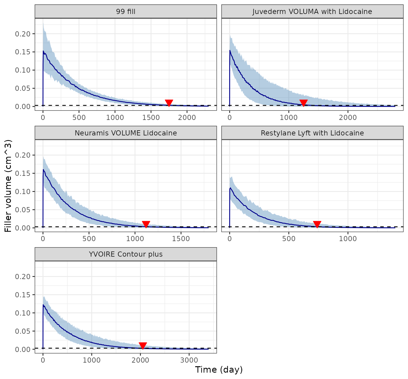
Replicates Figure 4 of Ryu 2021: simulated median (line) and 90% prediction interval (band) of filler volume, with the published Tcd (triangle).
PKNCA check of the typical profiles
The paper reports no NCA, so PKNCA is used to confirm the two
properties that follow from the structure: the terminal half-life of the
volume is log(2) / Kswell (the decline is
swelling-limited), and the area under the volume curve is
100 / Kdeg.
nca_conc <- typ |>
  filter(!is.na(central)) |>
  mutate(id = 1L, treatment = filler, central = pmax(central, 0))
nca_dose <- data.frame(
  treatment = levels(fillers$filler), id = 1L, time = 0, amt = 100
)
conc_obj <- PKNCA::PKNCAconc(nca_conc, central ~ time | treatment + id)
dose_obj <- PKNCA::PKNCAdose(nca_dose, amt ~ time | treatment + id)
intervals <- data.frame(
  start = 0, end = Inf,
  cmax = TRUE, tmax = TRUE, half.life = TRUE, aucinf.obs = TRUE
)
nca_res <- PKNCA::pk.nca(PKNCA::PKNCAdata(conc_obj, dose_obj, intervals = intervals))
nca_wide <- as.data.frame(nca_res$result) |>
  filter(PPTESTCD %in% c("cmax", "tmax", "half.life", "aucinf.obs")) |>
  select(treatment, PPTESTCD, PPORRES) |>
  tidyr::pivot_wider(names_from = PPTESTCD, values_from = PPORRES) |>
  mutate(filler = factor(treatment, levels = levels(fillers$filler))) |>
  left_join(select(tcd_check, filler, ka, kdeg) |>
    mutate(filler = factor(filler, levels = levels(fillers$filler))), by = "filler") |>
  mutate(
    thalf_theory = log(2) / ka,
    auc_theory = 100 / kdeg
  )
nca_wide |>
  select(filler, cmax, tmax, half.life, thalf_theory, aucinf.obs, auc_theory) |>
  dplyr::rename(
    "Filler" = filler,
    "Cmax (cm^3)" = cmax,
    "Tmax (day)" = tmax,
    "t1/2, PKNCA (day)" = half.life,
    "log(2)/Kswell (day)" = thalf_theory,
    "AUCinf, PKNCA (cm^3*day)" = aucinf.obs,
    "100/Kdeg (cm^3*day)" = auc_theory
  ) |>
knitr::kable(digits = 3)| Filler | Cmax (cm^3) | Tmax (day) | t1/2, PKNCA (day) | log(2)/Kswell (day) | AUCinf, PKNCA (cm^3*day) | 100/Kdeg (cm^3*day) |
|---|---|---|---|---|---|---|
| 99 fill | 0.150 | 4.5 | 315.068 | 315.067 | 68.964 | 68.966 |
| Juvederm VOLUMA with Lidocaine | 0.152 | 3.5 | 228.009 | 228.009 | 50.504 | 50.505 |
| Neuramis VOLUME Lidocaine | 0.160 | 3.0 | 195.253 | 195.253 | 45.454 | 45.455 |
| Restylane Lyft with Lidocaine | 0.111 | 1.5 | 146.234 | 146.234 | 23.585 | 23.585 |
| YVOIRE Contour plus | 0.123 | 4.5 | 380.851 | 380.850 | 68.026 | 68.027 |
Assumptions and deviations
-
Kswell scale. Table 1 prints Kswell under a
‘day^-1’ header; the models use the printed value times 10^-3 per day.
The deposited control stream initialises
KSWELLat 0.0036, and only this scale reproduces Table 2 and Figures 2 and 4 (sections above). Kdeg is used as printed. -
Dose record. The models are dosed with
amt = 100intodepot, the injected volume in uL, and return the volume in cm^3 with no conversion. This reproduces how the fit was run: the paper states that the injected and observed volumes ‘coincided in cm^3’, but the typical-value model only reproduces the published peaks and Tcd with a numeric dose of 100. Dosingamt = 0.1scales every predicted volume down by 1000. The Kswell and Kdeg values are therefore specific to this dose record and are not physical swelling and degradation rates in the usual sense: Kdeg governs the first-days rise, and Kswell the multi-year decline. -
Timing of the peak. With Kdeg near 1.5-4 per day
the typical volume peaks 1.5-4.5 days after injection, whereas the
observed means in Figure 2 peak between days 7 and 28. This follows from
the published estimates, not from the extraction: with
tpeak = log(Kdeg / Kswell) / (Kdeg - Kswell), a peak near day 14 would need Kdeg of about 0.3 per day. -
Compartment naming. The paper’s SC compartment,
which is the observed compartment, is
central, and Kswell, the first-order transfer out of the depot, is the canonical absorption rateka. -
IIV conversion. Table 1 gives IIV as a CV; it is
converted with
omega^2 = log(1 + CV^2). If the paper instead reportedsqrt(omega^2), the variances would be 1-10% larger (largest for Juvederm, 46.5%). - Structure for the four fillers without a deposited stream. Text S1 is the Neuramis control stream. Methods 2.2 and Table 1 show that the same structure (Equations 1-4, one random effect scaled onto Kdeg, proportional error) was fitted to every filler, and it is applied to all five.
- Figure read-offs. The Figure 4 peaks and Figure 2 day-480 means used as checks above were read from the published figures by the maintainers.