6-Mercaptopurine (Hawwa 2008)
Source:vignettes/articles/Hawwa_2008_mercaptopurine.Rmd
Hawwa_2008_mercaptopurine.RmdModel and source
- Citation: Hawwa AF, Collier PS, Millership JS, McCarthy A, Dempsey S, Cairns C, McElnay JC. Population pharmacokinetic and pharmacogenetic analysis of 6-mercaptopurine in paediatric patients with acute lymphoblastic leukaemia. Br J Clin Pharmacol. 2008;66(6):826-837.
- Article: https://doi.org/10.1111/j.1365-2125.2008.03281.x
The model describes oral 6-mercaptopurine (6-MP) and its two active
intracellular metabolites, 6-thioguanine nucleotides (6-TGNs) and
6-methylmercaptopurine nucleotides (6-mMPNs), measured in erythrocytes
(RBCs). The structural model is a one-compartment first-order absorption
+ first-order elimination representation for 6-MP – whose plasma
concentration is NOT observed – and two metabolite compartments fed by a
common metabolic flux kme = 0.78 * k20. The fractional split between
6-TGNs and 6-mMPNs is controlled by FM3; the only retained
covariates are the TPMT genotype (any TPMT3 mutation, pooled
binary) on FM3 (theta = 2.56) and body surface area on the
apparent clearance of 6-TGNs (theta = 1.16, anchored to BSA = 1 m^2).
The fixed structural anchors (ka, F, k20, kme/k20) are taken from the
prior 6-MP literature, and apparent volumes of distribution are not
identifiable from the RBC-sampling design and are fixed to 1 L by the
ADVAN6 implementation convention (see Errata below).
Population
The model was fit to 150 erythrocyte metabolite concentrations across
75 sampling occasions (one sample per occasion, up to five occasions per
patient) from 19 paediatric patients (6 female, 13 male) with acute
lymphoblastic leukaemia receiving maintenance 6-MP at a target dose of
75 mg/m^2/day with weekly methotrexate co-medication. Baseline
demographics from Hawwa 2008 Table 1: age 3 - 17 years (median 10), body
weight 13.2 - 77.5 kg (median 33.4), body surface area 0.59 - 2.00 m^2
(median 1.14). The TPMT3-mutation panel screened in the cohort
comprised TPMT3A (1 heterozygote / 0 homozygotes), TPMT3B (none
observed), and TPMT*3C (2 heterozygotes / 0 homozygotes). The same
information is available programmatically via
readModelDb("Hawwa_2008_mercaptopurine")$population.
Source trace
The per-parameter origin is recorded as an in-file comment next to
each ini() entry in
inst/modeldb/specificDrugs/Hawwa_2008_mercaptopurine.R. The
table below collects them in one place.
| Equation / parameter | Value | Source location |
|---|---|---|
lka |
log(1.3 1/h) FIXED | Methods page 4 (“ka was fixed at 1.3 1/h according to the literature [1, 9]”) |
lfdepot |
log(0.22) FIXED | Methods page 4 (bioavailability factor F fixed at 22% per literature [1, 9]) |
lvc |
log(1 L) FIXED | ADVAN6 implementation convention (6-MP plasma not observed; see Errata) |
lcl |
log(0.53 L/h) FIXED | Methods page 5 (k20 = 0.53 1/h per literature [1, 9]; CL = k20 * V_central) |
e_fmet |
0.78 FIXED | Methods page 5 (“k_other = 0.22 * k20”; so kme/k20 = 1 - 0.22 = 0.78) |
lvc_tgn |
log(1 L) FIXED | ADVAN6 implementation convention (not identifiable; see Errata) |
lcl_tgn |
log(0.00914 L/h) | Table 4 FINAL row CL 6-TGNs theta = 0.00914 L/h (SE 56.8%) |
lvc_mmpn |
log(1 L) FIXED | ADVAN6 implementation convention (not identifiable; see Errata) |
lcl_mmpn |
log(0.0228 L/h) | Table 4 FINAL row CL 6-mMPNs theta = 0.0228 L/h (SE 14.2%) |
lfm3 |
log(0.0191) | Table 4 FINAL row FM3 theta = 0.0191 (SE 64.1%) |
e_bsa_cl_tgn |
1.16 | Table 4 FINAL row BSA theta = 1.16 (SE 49.0%); equation CL_6TGNs = theta * BSA^1.16 |
e_tpmt_mut_fm3 |
log(2.56) | Table 4 FINAL row TPMT theta = 2.56 (SE 35.9%); equation TVFM3 = theta_FM3 * theta_TPMT^TPMT_MUT |
etalcl_tgn |
omega^2 = 0.113 | Table 4 FINAL row w_CL_6TGNs = 0.113 (sqrt = 33.6%, the reported CV%) |
etalcl_mmpn |
omega^2 = 0.11 | Table 4 FINAL row w_CL_6mMPNs = 0.11 (sqrt = 33.2%, the reported CV%) |
addSd_tgn |
0.177 mg/L | Table 4 FINAL row s_6TGNs = 0.177 mg/L (SE 17.5%) |
addSd_mmpn |
8.42 mg/L | Table 4 FINAL row s_6mMPNs = 8.42 mg/L (SE 19.3%) |
d/dt(depot) |
-ka * depot | Methods page 5 first ODE (explicit form of analytical ka * dose input) |
d/dt(central) |
kadepot - kelcentral | Methods page 5 second ODE; kel = cl/vc = k20 = 0.53 1/h |
d/dt(central_tgn) |
fm3 * kme * central - (cl_tgn/vc_tgn) * central_tgn | Methods page 5 third ODE for metabolite i=3 |
d/dt(central_mmpn) |
(1-fm3) * kme * central - (cl_mmpn/vc_mmpn) * central_mmpn | Methods page 5 fourth ODE; FM4 = 1 - FM3 |
f(depot) <- 0.22 |
bioavailability | Methods page 4 F = 22% fixed |
Virtual cohort
The original observed data are not publicly available. The simulation below uses 100 virtual paediatric patients whose body weight, body surface area, and TPMT genotype distributions approximate the Table 1 demographics (weight log-normal around the median 33.4 kg; BSA log-normal around the median 1.14 m^2; TPMT_MUT Bernoulli at 3/19 = 0.158 to match the cohort prevalence). Each patient receives a single daily oral 6-MP dose titrated to 75 mg/m^2/day (rounded to whole milligrams to match the Table 1 dose range of 10 - 100 mg).
set.seed(20081124)
n_subj <- 100L

subj <- tibble::tibble(
  id       = seq_len(n_subj),
  WT       = round(rlnorm(n_subj, meanlog = log(33.4), sdlog = 0.45), 1),
  BSA      = round(pmin(pmax(rlnorm(n_subj, meanlog = log(1.14), sdlog = 0.35),
                              0.59), 2.00), 2),
  TPMT_MUT = as.integer(runif(n_subj) < 3 / 19)
) |>
  dplyr::mutate(
    daily_dose_mg = round(pmin(pmax(75 * BSA, 10), 100))
  )

# Build the event table: daily dosing at t = 0, 24, ..., 24 * (n_days - 1) hours,
# with observation sampling every 6 h across the full simulation horizon (60
# days) so we can characterise both the approach to steady state and the
# steady-state plateau. cmt = "Cc_tgn" is a placeholder that triggers rxSolve
# to return every output column (Cc_tgn and Cc_mmpn) at each observation row.
n_days     <- 60L
dose_times <- seq(0, by = 24, length.out = n_days)
obs_times  <- seq(0, n_days * 24, by = 6)

make_one_subject <- function(i) {
  row <- subj[i, ]
  ev <- rxode2::et(amt = row$daily_dose_mg, cmt = "depot",
                   time = dose_times)
  ev <- rxode2::et(ev, time = obs_times, cmt = "Cc_tgn")
  ev <- as.data.frame(ev)
  ev$id       <- row$id
  ev$WT       <- row$WT
  ev$BSA      <- row$BSA
  ev$TPMT_MUT <- row$TPMT_MUT
  ev
}

events <- do.call(rbind, lapply(seq_len(nrow(subj)), make_one_subject))
stopifnot(!anyDuplicated(unique(events[, c("id", "time", "evid")])))
Simulation
mod <- readModelDb("Hawwa_2008_mercaptopurine")

sim <- rxode2::rxSolve(
  mod,
  events = events,
  keep   = c("WT", "BSA", "TPMT_MUT")
) |>
  as.data.frame()
For deterministic replication of typical-value trajectories (Figures 2 / 6 of the paper plot model-predicted concentrations from the FINAL population parameters), zero out the random effects.
mod_typ <- mod |> rxode2::zeroRe()Replicate published figures
Figure 1 – TPMT-mutant vs. wild-type metabolite profiles
Hawwa 2008 Figure 1 reports individual 6-TGN and 6-mMPN concentration-time profiles across the study period, with TPMT-mutant patients highlighted and generally showing higher 6-TGNs and lower 6-mMPNs than the wild-type patients. The simulation below shows the typical-value trajectories for a median patient (BSA = 1.14 m^2, daily dose 86 mg = 75 * 1.14 rounded) under TPMT wild-type vs. TPMT mutation.
median_subj <- function(tpmt_mut) {
  ev <- rxode2::et(amt = 86, cmt = "depot",
                   time = dose_times)
  ev <- rxode2::et(ev, time = obs_times, cmt = "Cc_tgn")
  ev <- as.data.frame(ev)
  ev$id       <- 1L
  ev$WT       <- 33.4
  ev$BSA      <- 1.14
  ev$TPMT_MUT <- as.integer(tpmt_mut)
  ev
}

typ_wt  <- rxode2::rxSolve(mod_typ, events = median_subj(0)) |> as.data.frame()
#> ℹ omega/sigma items treated as zero: 'etalcl_tgn', 'etalcl_mmpn'
typ_mut <- rxode2::rxSolve(mod_typ, events = median_subj(1)) |> as.data.frame()
#> ℹ omega/sigma items treated as zero: 'etalcl_tgn', 'etalcl_mmpn'

typ_long <- dplyr::bind_rows(
  typ_wt  |> dplyr::mutate(TPMT = "Wild-type"),
  typ_mut |> dplyr::mutate(TPMT = "Mutation (TPMT*3*)")
) |>
  dplyr::filter(time > 0) |>
  dplyr::transmute(
    time_days = time / 24,
    TPMT,
    `6-TGN (mg/L)`  = Cc_tgn,
    `6-mMPN (mg/L)` = Cc_mmpn
  ) |>
  tidyr::pivot_longer(
    cols      = c(`6-TGN (mg/L)`, `6-mMPN (mg/L)`),
    names_to  = "analyte",
    values_to = "conc"
  )

ggplot(typ_long, aes(time_days, conc, colour = TPMT)) +
  geom_line(linewidth = 0.9) +
  facet_wrap(~analyte, scales = "free_y") +
  labs(
    x       = "Time after first dose (days)",
    y       = "RBC concentration (mg/L)",
    colour  = "TPMT genotype",
    title   = "Figure 1 replication -- TPMT effect on metabolite trajectories",
    caption = "Typical-value (zeroRe) prediction for a median paediatric ALL patient (BSA = 1.14 m^2, daily oral 6-MP 86 mg)."
  )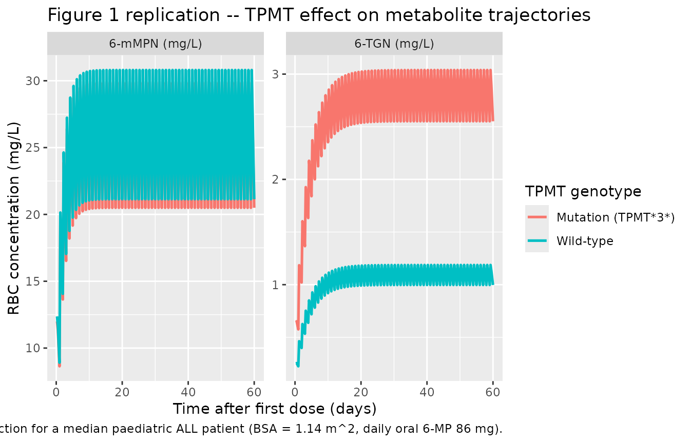
The simulation reproduces the qualitative pattern reported by Hawwa
2008: a TPMT3 mutation raises the 6-TGN steady-state plateau by
~2.56-fold via the multiplicative effect on FM3, and lowers the 6-mMPN
steady-state plateau by ~3% (because the complementary fraction
1 - FM3 falls from 0.981 to 0.951 when TPMT_MUT = 1).
Steady-state mean comparison vs. paper page 829
Hawwa 2008 reports the mean RBC concentrations across the FULL dataset (index + validation, 19 patients, 75 samples, 150 concentrations) as 0.729 mg/L (6-TGN) and 14.61 mg/L (6-mMPN). The simulation below computes the population-averaged mean of each metabolite over the steady-state window (days 30 - 60) and compares to those reference means.
sim_ss <- sim |>
  dplyr::filter(time >= 30 * 24, time <= 60 * 24) |>
  dplyr::group_by(id) |>
  dplyr::summarise(
    mean_tgn  = mean(Cc_tgn,  na.rm = TRUE),
    mean_mmpn = mean(Cc_mmpn, na.rm = TRUE),
    .groups   = "drop"
  )

published_mean <- tibble::tibble(
  analyte         = c("6-TGN", "6-mMPN"),
  paper_mean      = c(0.729,  14.61)
)

sim_summary <- tibble::tibble(
  analyte         = c("6-TGN", "6-mMPN"),
  sim_mean        = c(mean(sim_ss$mean_tgn),  mean(sim_ss$mean_mmpn)),
  sim_p05         = c(quantile(sim_ss$mean_tgn,  0.05),
                      quantile(sim_ss$mean_mmpn, 0.05)),
  sim_p95         = c(quantile(sim_ss$mean_tgn,  0.95),
                      quantile(sim_ss$mean_mmpn, 0.95))
)

sim_summary |>
  dplyr::left_join(published_mean, by = "analyte") |>
  dplyr::transmute(
    Analyte                       = analyte,
    `Simulated mean (mg/L)`       = sprintf("%.3f", sim_mean),
    `Simulated 5%-95% (mg/L)`     = sprintf("%.3f - %.3f", sim_p05, sim_p95),
    `Hawwa 2008 mean (mg/L)`      = sprintf("%.3f", paper_mean),
    `Relative difference (%)`     = sprintf("%+.1f",
                                            100 * (sim_mean - paper_mean) / paper_mean)
  ) |>
  knitr::kable(
    caption = "Simulated steady-state mean RBC metabolite concentrations (days 30 - 60, 100 virtual patients) vs. the full-dataset cohort means reported in Hawwa 2008 Results.",
    align   = c("l", "r", "r", "r", "r")
)| Analyte | Simulated mean (mg/L) | Simulated 5%-95% (mg/L) | Hawwa 2008 mean (mg/L) | Relative difference (%) |
|---|---|---|---|---|
| 6-TGN | 1.381 | 0.492 - 2.818 | 0.729 | +89.5 |
| 6-mMPN | 24.777 | 10.443 - 45.527 | 14.610 | +69.6 |
BSA sensitivity (paper page 826)
Hawwa 2008 reports that the BSA power-law on CL_6TGNs spans 0.0049 - 0.0204 L/h across the cohort BSA range of 0.59 - 2.00 m^2 (page 826). The sensitivity sweep below reproduces that range from the packaged model directly, without re-solving the ODEs.
cl_tgn_at_BSA1 <- 0.00914
bsa_grid <- c(0.59, 0.80, 1.14, 1.50, 2.00)
sim_cl <- tibble::tibble(
  BSA              = bsa_grid,
  `CL_6TGNs (L/h)` = cl_tgn_at_BSA1 * BSA^1.16
)

paper_range <- tibble::tibble(
  BSA              = c(0.59, 2.00),
  `CL_6TGNs (L/h)` = c(0.0049, 0.0204)
)

sim_cl |>
  dplyr::left_join(paper_range, by = "BSA",
                   suffix = c("", " (Hawwa 2008 page 826)")) |>
  knitr::kable(
    caption = "BSA power-law sensitivity for CL_6TGNs. The packaged formula reproduces the paper's reported 0.005 - 0.02 L/h range across BSA 0.59 - 2.00 m^2.",
    digits  = c(2, 4, 4)
)| BSA | CL_6TGNs (L/h) | CL_6TGNs (L/h) (Hawwa 2008 page 826) |
|---|---|---|
| 0.59 | 0.0050 | 0.0049 |
| 0.80 | 0.0071 | NA |
| 1.14 | 0.0106 | NA |
| 1.50 | 0.0146 | NA |
| 2.00 | 0.0204 | 0.0204 |
PKNCA single-dose check
For a sanity NCA on a single 50 mg oral 6-MP dose to a median patient (BSA = 1.14, TPMT wild-type), the packaged model is evaluated with PKNCA over the first 28 days post-dose (the metabolite half-lives are long enough that single-dose AUC is dominated by the slow elimination phase rather than the absorption peak). Because Hawwa 2008 does not report population NCA values directly, this section is a structural sanity check rather than a published- vs-simulated comparison.
pknca_events <- {
  ev <- rxode2::et(amt = 50, cmt = "depot", time = 0)
  ev <- rxode2::et(ev, time = seq(0, 28 * 24, by = 2), cmt = "Cc_tgn")
  ev <- as.data.frame(ev)
  ev$id       <- 1L
  ev$WT       <- 33.4
  ev$BSA      <- 1.14
  ev$TPMT_MUT <- 0L
  ev
}

sim_sd <- rxode2::rxSolve(mod_typ, events = pknca_events) |>
  as.data.frame()
#> ℹ omega/sigma items treated as zero: 'etalcl_tgn', 'etalcl_mmpn'
# Single-subject rxSolve drops the `id` column; reinstate it for the PKNCA
# objects below.
if (!"id" %in% names(sim_sd)) sim_sd$id <- 1L
sim_nca_tgn <- sim_sd |>
  dplyr::filter(!is.na(Cc_tgn)) |>
  dplyr::transmute(id, time, Cc = Cc_tgn, treatment = "6-TGN")

dose_df_tgn <- pknca_events |>
  dplyr::filter(evid == 1) |>
  dplyr::transmute(id, time, amt, treatment = "6-TGN")

sim_nca_tgn <- dplyr::bind_rows(
  sim_nca_tgn,
  sim_nca_tgn |>
    dplyr::distinct(id, treatment) |>
    dplyr::mutate(time = 0, Cc = 0)
) |>
  dplyr::distinct(id, treatment, time, .keep_all = TRUE) |>
  dplyr::arrange(id, treatment, time)

conc_obj_tgn <- PKNCA::PKNCAconc(
  sim_nca_tgn, Cc ~ time | treatment + id,
  concu = "mg/L", timeu = "h"
)
dose_obj_tgn <- PKNCA::PKNCAdose(
  dose_df_tgn, amt ~ time | treatment + id,
  doseu = "mg"
)

intervals <- data.frame(
  start       = 0,
  end         = Inf,
  cmax        = TRUE,
  tmax        = TRUE,
  aucinf.obs  = TRUE,
  half.life   = TRUE
)

nca_tgn <- PKNCA::pk.nca(
  PKNCA::PKNCAdata(conc_obj_tgn, dose_obj_tgn, intervals = intervals)
)
knitr::kable(summary(nca_tgn),
caption = "6-TGN simulated single-dose NCA (50 mg oral 6-MP, BSA = 1.14, TPMT wild-type).")| Interval Start | Interval End | treatment | N | Cmax (mg/L) | Tmax (h) | Half-life (h) | AUCinf,obs (h*mg/L) |
|---|---|---|---|---|---|---|---|
| 0 | Inf | 6-TGN | 1 | 0.151 | 8.00 | 65.1 | 15.4 |
sim_nca_mmpn <- sim_sd |>
  dplyr::filter(!is.na(Cc_mmpn)) |>
  dplyr::transmute(id, time, Cc = Cc_mmpn, treatment = "6-mMPN")

dose_df_mmpn <- pknca_events |>
  dplyr::filter(evid == 1) |>
  dplyr::transmute(id, time, amt, treatment = "6-mMPN")

sim_nca_mmpn <- dplyr::bind_rows(
  sim_nca_mmpn,
  sim_nca_mmpn |>
    dplyr::distinct(id, treatment) |>
    dplyr::mutate(time = 0, Cc = 0)
) |>
  dplyr::distinct(id, treatment, time, .keep_all = TRUE) |>
  dplyr::arrange(id, treatment, time)

conc_obj_mmpn <- PKNCA::PKNCAconc(
  sim_nca_mmpn, Cc ~ time | treatment + id,
  concu = "mg/L", timeu = "h"
)
dose_obj_mmpn <- PKNCA::PKNCAdose(
  dose_df_mmpn, amt ~ time | treatment + id,
  doseu = "mg"
)

nca_mmpn <- PKNCA::pk.nca(
  PKNCA::PKNCAdata(conc_obj_mmpn, dose_obj_mmpn, intervals = intervals)
)
knitr::kable(summary(nca_mmpn),
caption = "6-mMPN simulated single-dose NCA (50 mg oral 6-MP, BSA = 1.14, TPMT wild-type).")| Interval Start | Interval End | treatment | N | Cmax (mg/L) | Tmax (h) | Half-life (h) | AUCinf,obs (h*mg/L) |
|---|---|---|---|---|---|---|---|
| 0 | Inf | 6-mMPN | 1 | 7.25 | 8.00 | 30.4 | 369 |
Assumptions and deviations
-
Apparent metabolite volumes fixed to 1 L (not
identifiable). Hawwa 2008 parameterises each metabolite
compartment through an apparent clearance alone; the apparent
distribution volume is not identifiable from the RBC sampling design
(one sample per occasion, up to 5 occasions per patient across several
months) and the NONMEM ADVAN6 implementation conventionally treats the
metabolite compartment as having unit apparent volume so the reported
clearance acts effectively as a first-order rate constant. At steady
state the metabolite concentration depends only on the
metabolite-formation flux (driven by FM3 and kme) divided by the
apparent clearance and is independent of the apparent volume; the only
dynamic consequence of the V = 1 L convention is the half-life used to
reach steady state (~63 h for 6-TGN, ~30 h for 6-mMPN). The same
convention is used by
inst/modeldb/specificDrugs/Urien_2005_capecitabine.Rfor the three capecitabine metabolites with the same ADVAN6 structure. - 6-MP central volume V_central also fixed to 1 L. 6-MP plasma concentration is NOT observed in this study; only the RBC metabolites are measured. The 6-MP central compartment carries only the transient absorption / first-order-elimination dynamics that feed the two metabolite compartments. With V_central = 1 L fixed by the same convention, the apparent CL_central = 0.53 L/h reproduces the paper’s k20 = 0.53 1/h exactly when CL/V is the elimination rate constant.
-
kme / k20 ratio fixed at 0.78. Hawwa 2008 Methods
page 5 states “k_other = 0.22 * k20 = 0.1166 1/h based on the literature
[9]” and “k20 = kme + k_other”, which together imply kme = (1 - 0.22) *
k20 = 0.78 * k20 = 0.4134 1/h. The model file declares this as the
explicit fixed structural anchor
e_fmet = 0.78(the metabolic fraction of total 6-MP elimination); the complementaryk_otherarm is consumed by the central -> outside elimination pathway and is not tracked as a separate compartment because it does not feed any observed concentration. -
TPMT genotyping panel pooled into a single binary.
Hawwa 2008 Table 1 reports cohort genotyping at three TPMT3
variants (TPMT3A, TPMT3B, TPMT*3C). The cohort was too small (n
= 19; 3 heterozygote carriers across the three variants combined) to
estimate per-allele effects, so the source paper pools all three into a
single binary indicator denoted
TPMTin Table 4 and defined in the table footer as “TPMT = 1 if the patient had any TPMT mutation, 0 otherwise”. The packaged model carries the same pooled binary under the canonical column nameTPMT_MUT; downstream users with panel-resolved genotypes should preserve the pooled orientation (TPMT_MUT = 1if any reduced-function allele is observed across whichever variants the user’s panel assays). - **TPMT*2 not assayed.** The Hawwa 2008 cohort was not genotyped at TPMT2 (rs1800462, A80P). Subjects carrying TPMT2 (a rarer variant) would be misclassified as wild-type in this panel; in practice the TPMT*2 allele frequency in European cohorts is ~0.4% so the misclassification rate is very low.
-
XO and ITPA polymorphisms screened but not
retained. The source paper screened TWO polymorphisms in
xanthine oxidase (XO A1936G and A2107G) and TWO in inosine
triphosphatase (ITPA C94A and IVS2+21A>C). None reached the
OFV-retention threshold (delta OBJF >= 6.63, p < 0.01) in the
FINAL covariate model and they are not represented in this file. The
model file’s
population$notesrecords the screening for downstream provenance. - Bayesian individual estimates vs. typical predictions. Hawwa 2008 Table 5 reports the median individual Bayesian post-hoc estimates of FM3 (0.0191 wild-type / 0.0491 mutant), CL_6TGNs (0.0112 L/h), and CL_6mMPNs (0.0226 L/h). These are population-pooled summaries of the individual posterior modes; the typical-value population predictions implemented in this file reproduce the Table 4 FINAL theta point estimates directly (FM3 = 0.0191 WT, CL_6TGNs at BSA = 1 m^2 = 0.00914 L/h, CL_6mMPNs = 0.0228 L/h). For the median patient (BSA = 1.14 m^2) the typical-value CL_6TGNs is 0.00914 * 1.14^1.16 = 0.0107 L/h, close to the 0.0112 L/h Bayesian-median estimate; the small discrepancy reflects the difference between the population typical value at a single covariate point vs. the median across a distribution of individual posterior modes.
- No IIV on FM3. The FINAL model retained IIV only on CL_6TGNs and CL_6mMPNs; the FM3 parameter is a typical-value structural quantity with no eta term. Stochastic simulations therefore underpredict the individual-level spread in the metabolite-formation fraction; the population-averaged predictions are unaffected.
- Pediatric / adult applicability. The model was developed in paediatric ALL patients on maintenance 6-MP (target 75 mg/m^2/day) with weekly methotrexate co-medication. Extrapolation to adult ALL, inflammatory bowel disease 6-MP / azathioprine use, or paediatric patients outside the cohort BSA range (0.59 - 2.00 m^2) is not supported by the source data.