Nafamostat: intravenous PK with unbound and lung outputs (Jeong 2022)
Source:vignettes/articles/Jeong_2022_nafamostat.Rmd
Jeong_2022_nafamostat.RmdModel and source
mod <- readModelDb("Jeong_2022_nafamostat")
ui <- rxode2::rxode(mod)- Citation: Jeong HC, Chae YJ, Shin KH. (2022). Predicting the systemic exposure and lung concentration of nafamostat using physiologically-based pharmacokinetic modeling. Transl Clin Pharmacol 30(4):201-211. doi:10.12793/tcp.2022.30.e20.
- Article: https://doi.org/10.12793/tcp.2022.30.e20 (open access, https://www.ncbi.nlm.nih.gov/pmc/articles/PMC9810492/)
What this model is, and what it is not
Jeong 2022 builds a Simcyp (version 21) physiologically based pharmacokinetic (PBPK) model of nafamostat, an intravenous serine-protease inhibitor that is hydrolysed rapidly by plasma and tissue esterases. The model is verified against 2-h intravenous infusions of 10, 20 and 40 mg in healthy Chinese volunteers (Cao et al. 2008, reference 22). It is then applied to two continuous-infusion regimens proposed for COVID-19: 200 mg/24 h and 4.8 mg/kg/24 h, each for 13 days. For both regimens the paper predicts the total and unbound plasma concentrations and the total lung-tissue concentration.
Simcyp’s whole-body equations are proprietary and do not appear in
the paper. Distribution uses the full-PBPK layout, with Rodgers and
Rowland partition coefficients multiplied by an estimated
Kp scalar of 2.18. Elimination is built from CES2 enzyme
kinetics, a plasma esterase half-life, additional liver microsomal and
cytosolic intrinsic clearances, renal clearance and an additional
systemic clearance (Table 1). Converting those inputs into a systemic
clearance needs unpublished Simcyp system values: microsomal and
cytosolic protein per gram of liver, liver weight and plasma volume. The
organ volumes, blood flows and per-tissue Kp values are not
printed either. The platform model itself therefore cannot be
encoded.
The paper does publish enough output to determine an intravenous reduction:
-
Table 2 gives the PBPK model’s predicted mean
AUC0-inf at three doses. Dose / AUC0-inf is 220.8 L/h at every dose, so
this is the model’s clearance, and nafamostat is dose-linear over 10-40
mg (the CES2
Kmof 1,790 uM is far above any plasma concentration). - Table 1 gives the predicted steady-state volume, 11.66 L/kg.
- Figure 1 plots the predicted mean plasma profile for each dose over 8 h. The figures in the article PDF are vector graphics, so the curves were read from their path coordinates rather than by eye. The digitised apexes reproduce the Table 2 predicted Cmax (18.5, 36.9 and 73.9 ng/mL) to within 0.6%.
- Figure 2 plots the predicted total plasma, unbound plasma and lung profiles over the 13-day infusions.
The reduction fixes clearance at 220.8 L/h and the total volume at 11.66 L/kg x 70 kg. It recovers the remaining distribution constants from Figure 1 alone and holds out Table 2’s Cmax and AUC0-last and all of Figure 2 as independent checks.
Population
p <- ui$population
pop_tab <- tibble::tibble(
  Field = c("Species", "Virtual subjects", "Age", "% female", "Population",
            "Doses"),
  Value = c(p$species, p$n_subjects, p$age_range, p$sex_female_pct,
            p$race_ethnicity, p$dose_range)
)
knitr::kable(pop_tab, caption = "Simulated population (Jeong 2022 Methods).")| Field | Value |
|---|---|
| Species | human |
| Virtual subjects | 1000 |
| Age | 20-40 years (virtual healthy volunteers; the clinical verification study enrolled healthy Chinese adults aged 20-30 years) |
| % female | 50 |
| Population | Simcyp virtual healthy-volunteer population; verification data from healthy Chinese adults |
| Doses | Verification: single 2-h intravenous infusions of 10, 20 and 40 mg. Application: continuous intravenous infusion of 200 mg/24 h or 4.8 mg/kg/24 h for 13 days. |
The clinical verification study (Cao et al. 2008) enrolled 10 healthy Chinese volunteers per dose, aged 20-30 years, with the sex ratio not reported. The simulations used 10 virtual trials of 100 subjects aged 20-40 years with a 50:50 sex ratio. No body weight is reported for either the clinical or the virtual population.
Source trace
Every value in the ini() block, with its source
location.
trace_tab <- tibble::tribble(
  ~Parameter, ~Value,       ~Source,
  "lcl",      "220.8 L/h",  "Table 2 predicted AUC0-inf: 10 mg / 45.30, 20 mg / 90.60, 40 mg / 181.00 ng*h/mL",
  "lvc",      "7.61 L",     "Recovered from the Figure 1 predicted mean curves (joint fit, three doses)",
  "lq",       "104 L/h",    "Recovered from Figure 1",
  "lvp",      "42.2 L",     "Recovered from Figure 1",
  "lq2",      "64.8 L/h",   "Recovered from Figure 1",
  "lvp2",     "232 L",      "Recovered from Figure 1",
  "lq3",      "7.57 L/h",   "Recovered from Figure 1",
  "lvp3",     "534.4 L",    "Table 1 'Vss (L/kg)' 11.66 x 70 kg = 816.2 L, minus vc + vp + vp2",
  "fu",       "0.46",       "Table 1 'fu' (predicted in Simcyp)",
  "lkp_lung", "5.44",       "Ratio of the Figure 2C lung curve to the Figure 2A plasma curve",
  "propSd",   "0 (fixed)",  "No residual-error model is reported anywhere in the source"
)
knitr::kable(trace_tab, caption = "Source trace for every fixed parameter.")| Parameter | Value | Source |
|---|---|---|
| lcl | 220.8 L/h | Table 2 predicted AUC0-inf: 10 mg / 45.30, 20 mg / 90.60, 40 mg / 181.00 ng*h/mL |
| lvc | 7.61 L | Recovered from the Figure 1 predicted mean curves (joint fit, three doses) |
| lq | 104 L/h | Recovered from Figure 1 |
| lvp | 42.2 L | Recovered from Figure 1 |
| lq2 | 64.8 L/h | Recovered from Figure 1 |
| lvp2 | 232 L | Recovered from Figure 1 |
| lq3 | 7.57 L/h | Recovered from Figure 1 |
| lvp3 | 534.4 L | Table 1 ‘Vss (L/kg)’ 11.66 x 70 kg = 816.2 L, minus vc + vp + vp2 |
| fu | 0.46 | Table 1 ‘fu’ (predicted in Simcyp) |
| lkp_lung | 5.44 | Ratio of the Figure 2C lung curve to the Figure 2A plasma curve |
| propSd | 0 (fixed) | No residual-error model is reported anywhere in the source |
The model equations are the standard four-compartment mammillary
intravenous system. The outputs are
Cc = 1000 * central / vc (mg/L to ng/mL), the unbound
concentration Cu = fu * Cc, and the lung-tissue
concentration Clung = kp_lung * Cc. Both of the last two
are algebraic: the unbound fraction is a constant in the source (Table
1), and Figure 2 shows the lung concentration at a constant 5.440 times
plasma at every plotted time in both regimens. The lung receives the
whole cardiac output and is perfusion-limited, so it equilibrates with
plasma within minutes.
theta <- ui$theta
cl_mod  <- exp(theta[["lcl"]])
vss_mod <- exp(theta[["lvc"]]) + exp(theta[["lvp"]]) + exp(theta[["lvp2"]]) +
  exp(theta[["lvp3"]])
auc_inf_pred <- c(`10` = 45.30, `20` = 90.60, `40` = 181.00)  # Table 2
cl_implied <- 1000 * c(10, 20, 40) / auc_inf_pred
stopifnot(
  max(abs(cl_implied / cl_mod - 1)) < 0.001,
  abs(vss_mod / (11.66 * 70) - 1) < 0.001,
  theta[["fu"]] == 0.46
)
knitr::kable(
  tibble::tibble(Dose_mg = c(10, 20, 40), AUCinf = auc_inf_pred,
                 CL_implied = round(cl_implied, 2)) |>
    dplyr::rename("Dose (mg)" = Dose_mg,
                  "Predicted AUC0-inf (ng*h/mL)" = AUCinf,
                  "Dose / AUC0-inf (L/h)" = CL_implied),
  caption = "Clearance implied by the Table 2 predictions."
)| Dose (mg) | Predicted AUC0-inf (ng*h/mL) | Dose / AUC0-inf (L/h) |
|---|---|---|
| 10 | 45.3 | 220.75 |
| 20 | 90.6 | 220.75 |
| 40 | 181.0 | 220.99 |
Digitised reference curves
The predicted mean curves of Figures 1 and 2, read from the vector paths of the article PDF. Figure 1 is on a log axis (0.1-100 or 0.1-1,000 ng/mL over 0-8 h); Figure 2 is on linear nM axes with a break between days 2 and 8. On Figure 2’s day-scale axis the first 1.5 h of infusion spans less than two points of drawing width, so the rise is not resolvable there and the reference points start at 3 h.
mw <- 347.378  # g/mol, Table 1

fig1_t <- c(0.25, 0.5, 1, 1.5, 2, 2.05, 2.1, 2.25, 2.5, 3, 4, 5, 6, 7, 8)
fig1_ref <- dplyr::bind_rows(
  tibble::tibble(dose = 10, time = fig1_t, Cc_ref = c(
    14.051, 15.685, 16.994, 17.845, 18.475, 7.032, 5.934, 4.449, 3.306,
    2.207, 1.377, 0.987, 0.769, 0.634, 0.540)),
  tibble::tibble(dose = 20, time = fig1_t, Cc_ref = c(
    28.657, 31.467, 34.028, 35.722, 36.949, 13.537, 11.596, 8.771, 6.547,
    4.386, 2.743, 1.967, 1.535, 1.266, 1.079)),
  tibble::tibble(dose = 40, time = fig1_t, Cc_ref = c(
    56.496, 62.151, 67.737, 71.061, 73.552, 27.765, 23.729, 17.515, 13.006,
    8.821, 5.421, 3.937, 3.073, 2.509, 2.138))
)

fig2_t <- c(3, 6, 9, 13, 18, 24, 31, 39, 48, 192, 312)
fig2_ref <- dplyr::bind_rows(
  tibble::tibble(regimen = "200 mg/24 h", output = "Total plasma", time = fig2_t,
                 nM_ref = c(92.9, 98.6, 102.4, 105.7, 108.3, 110.2, 111.4, 112.2, 112.6, 113.0, 113.1)),
  tibble::tibble(regimen = "200 mg/24 h", output = "Unbound plasma", time = fig2_t,
                 nM_ref = c(42.1, 44.7, 46.4, 47.9, 49.1, 49.9, 50.5, 50.8, 51.0, 51.2, 51.2)),
  tibble::tibble(regimen = "200 mg/24 h", output = "Lung tissue", time = fig2_t,
                 nM_ref = c(505.5, 536.3, 557.2, 575.0, 589.1, 599.3, 606.1, 610.2, 612.4, 614.7, 615.3)),
  tibble::tibble(regimen = "4.8 mg/kg/24 h", output = "Total plasma", time = fig2_t,
                 nM_ref = c(136.1, 144.6, 150.2, 154.9, 158.6, 161.3, 163.3, 164.6, 165.5, 166.1, 166.3)),
  tibble::tibble(regimen = "4.8 mg/kg/24 h", output = "Unbound plasma", time = fig2_t,
                 nM_ref = c(61.9, 65.7, 68.2, 70.4, 72.1, 73.4, 74.3, 74.8, 75.1, 75.6, 75.7)),
  tibble::tibble(regimen = "4.8 mg/kg/24 h", output = "Lung tissue", time = fig2_t,
                 nM_ref = c(743.7, 789.0, 819.8, 846.0, 866.7, 881.7, 891.8, 897.8, 901.1, 904.6, 905.5))
)
Why four compartments
After each 2-h infusion the Figure 1 curves drop about 60% within three minutes, then fall with half-lives near 0.4 h and 3 h. The 11.66 L/kg volume also needs a deep, slowly equilibrating space. With clearance and Vss held at the same two anchors, the best two- and three-compartment reductions miss Figure 1 with log-scale RMSE of 0.37 and 0.085, against 0.050 here. They miss the 10 mg Table 2 Cmax by -14% and -10%; this model misses it by -0.6%. The four-compartment model’s half-lives follow.
k <- with(as.list(exp(theta[c("lcl", "lvc", "lq", "lvp", "lq2", "lvp2",
                              "lq3", "lvp3")])),
          c(kel = lcl / lvc, k12 = lq / lvc, k21 = lq / lvp,
            k13 = lq2 / lvc, k31 = lq2 / lvp2, k14 = lq3 / lvc,
            k41 = lq3 / lvp3))
A <- with(as.list(k), rbind(
  c(-(kel + k12 + k13 + k14), k21, k31, k41),
  c(k12, -k21, 0, 0),
  c(k13, 0, -k31, 0),
  c(k14, 0, 0, -k41)
))
thalf <- sort(log(2) / -Re(eigen(A)$values))
knitr::kable(tibble::tibble(Phase = 1:4, `Half-life (h)` = signif(thalf, 3)),
caption = "Disposition half-lives of the reduction.")| Phase | Half-life (h) |
|---|---|
| 1 | 0.0131 |
| 2 | 0.3820 |
| 3 | 3.2200 |
| 4 | 50.6000 |
The terminal half-life of about 50 h belongs to the deep compartment that carries most of the 816 L Vss. It holds little of a 2-h dose. AUC beyond 8 h is about 8% of AUC0-inf, which matches Table 2, where AUC0-last is 92% of AUC0-inf at every dose. That deep compartment also drives the slow approach to plateau over the first two days of the Figure 2 infusions.
Virtual cohort
The model has no random effects, so it is deterministic. One subject per regimen fully describes each arm.
- Verification arms: 10, 20 and 40 mg as 2-h infusions, observed to 14 days so that PKNCA can estimate AUC0-inf.
- COVID-19 arms: 200 mg/24 h and 4.8 mg/kg/24 h for 13 days. The paper does not print the body weight behind the per-kilogram regimen. Because this reduction has an absolute clearance, the ratio of the two Figure 2 plateaus (166.3 / 113.1 = 1.470) fixes the implied daily dose at 1.470 x 200 mg = 294 mg, or 4.8 mg/kg at 61.3 kg. That weight is used only to convert this regimen into an infusion rate.
Observations are placed on the central ODE state;
Cc, Cu and Clung are returned as
algebraic outputs on those rows.
wt_covid <- 1.470 * 200 / 4.8   # kg, from the Figure 2 plateau ratio

regimens <- tibble::tribble(
  ~arm,              ~dose_mg,           ~dur_h,  ~t_end,
  "10 mg over 2 h",  10,                 2,       336,
  "20 mg over 2 h",  20,                 2,       336,
  "40 mg over 2 h",  40,                 2,       336,
  "200 mg/24 h",     200 * 13,           24 * 13, 24 * 13,
  "4.8 mg/kg/24 h",  4.8 * wt_covid * 13, 24 * 13, 24 * 13
) |>
  dplyr::mutate(id = dplyr::row_number())

make_infusion <- function(id, arm, dose_mg, dur_h, t_end) {
  obs_grid <- sort(unique(c(
    seq(0, 3, by = 0.01), seq(3, 48, by = 0.25), seq(48, t_end, by = 2),
    fig1_t, fig2_t[fig2_t <= t_end], t_end
  )))
  dplyr::bind_rows(
    tibble::tibble(id = id, time = 0, amt = dose_mg, rate = dose_mg / dur_h,
                   evid = 1L, cmt = "central", arm = arm),
    tibble::tibble(id = id, time = obs_grid, amt = NA_real_, rate = NA_real_,
                   evid = 0L, cmt = "central", arm = arm)
  )
}

events <- regimens |>
  dplyr::rowwise() |>
  dplyr::reframe(make_infusion(id, arm, dose_mg, dur_h, t_end)) |>
  dplyr::arrange(id, time, dplyr::desc(evid))

stopifnot(!anyDuplicated(events[, c("id", "time", "evid")]),
sum(events$evid == 1L) == 5L)Replicate published figures
Figure 1: 2-h infusions of 10, 20 and 40 mg
sim_f1 <- sim |>
  dplyr::filter(arm %in% c("10 mg over 2 h", "20 mg over 2 h",
                           "40 mg over 2 h"), time <= 8) |>
  dplyr::mutate(dose = as.numeric(sub(" mg.*", "", arm)))

ggplot(sim_f1, aes(time, Cc)) +
  geom_line(colour = "steelblue4", linewidth = 0.7) +
  geom_point(data = fig1_ref, aes(time, Cc_ref), shape = 1, size = 1.8) +
  facet_wrap(~ dose, labeller = labeller(dose = \(x) paste(x, "mg"))) +
  scale_y_log10(limits = c(0.1, 1000)) +
  labs(x = "Time (h)", y = "Plasma nafamostat (ng/mL)",
       caption = paste("Replicates Figure 1A-C of Jeong 2022.",
                       "Line: reduction. Circles: published PBPK predicted mean.")) +
  theme_bw()
#> Warning in scale_y_log10(limits = c(0.1, 1000)): log-10 transformation
#> introduced infinite values.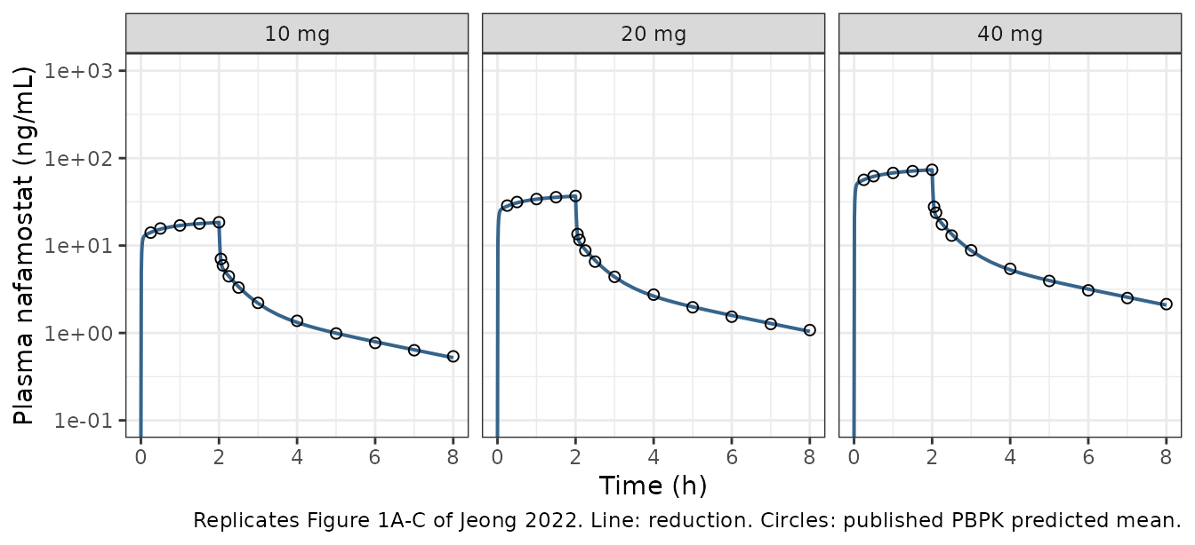
f1_cmp <- fig1_ref |>
  dplyr::mutate(arm = paste(dose, "mg over 2 h"), time = round(time, 6)) |>
  dplyr::left_join(sim |> dplyr::select(arm, time, Cc), by = c("arm", "time")) |>
  dplyr::mutate(pct = 100 * (Cc / Cc_ref - 1))
stopifnot(!anyNA(f1_cmp$Cc))
# These points were fitted, so this measures the quality of the reduction,
# not an independent validation. Median and 90th percentile, not the extreme:
# the curves are steep around the end of infusion, where a sub-point error in
# reading time moves the concentration most.
stopifnot(abs(median(f1_cmp$pct)) < 5,
          quantile(abs(f1_cmp$pct), 0.9) < 10)
knitr::kable(
  f1_cmp |>
    dplyr::group_by(dose) |>
    dplyr::summarise(median_pct = round(median(pct), 1),
                     max_abs_pct = round(max(abs(pct)), 1)) |>
    dplyr::rename("Dose (mg)" = dose, "Median % diff" = median_pct,
                  "Max |% diff|" = max_abs_pct),
  caption = "Reduction vs. the Figure 1 predicted mean curves (fitted points)."
)| Dose (mg) | Median % diff | Max |% diff| |
|---|---|---|
| 10 | -0.2 | 8.2 |
| 20 | -0.3 | 6.1 |
| 40 | 0.0 | 8.2 |
Figure 2: 13-day continuous infusions (held out)
None of these points was used to build the model.
sim_f2 <- sim |>
  dplyr::filter(arm %in% c("200 mg/24 h", "4.8 mg/kg/24 h")) |>
  dplyr::transmute(regimen = arm, time,
                   `Total plasma` = Cc / mw * 1000,
                   `Unbound plasma` = Cu / mw * 1000,
                   `Lung tissue` = Clung / mw * 1000) |>
  tidyr::pivot_longer(-c(regimen, time), names_to = "output",
                      values_to = "nM") |>
  dplyr::mutate(output = factor(output, c("Total plasma", "Unbound plasma",
                                          "Lung tissue")))

ggplot(sim_f2, aes(time / 24, nM)) +
  annotate("rect", xmin = -Inf, xmax = Inf, ymin = 30, ymax = 240,
           fill = "lightblue", alpha = 0.4) +
  geom_hline(yintercept = 10, linetype = "dashed", colour = "grey40") +
  geom_line(colour = "steelblue4", linewidth = 0.7) +
  geom_point(data = fig2_ref |>
               dplyr::mutate(output = factor(output, levels(sim_f2$output))),
             aes(time / 24, nM_ref), shape = 1, size = 1.6) +
  facet_grid(regimen ~ output) +
  labs(x = "Days", y = "Nafamostat (nM)",
       caption = paste("Replicates Figure 2A-F of Jeong 2022. Band: proposed",
                       "therapeutic range 30-240 nM; dashed: in vitro IC50",
                       "about 10 nM.\nCircles: published PBPK predicted mean.")) +
  theme_bw()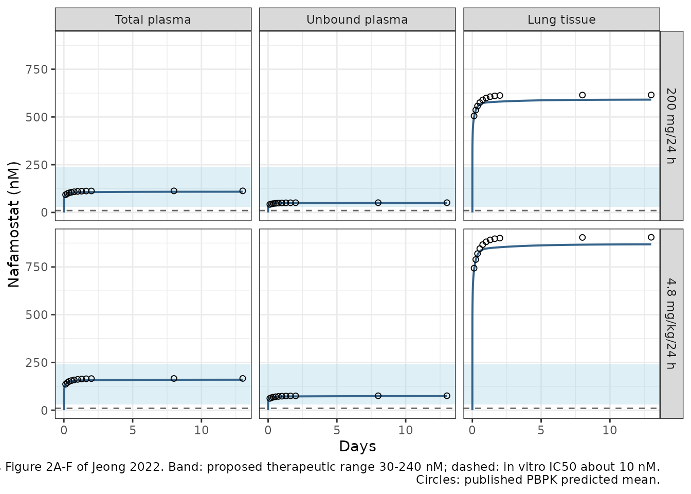
f2_cmp <- fig2_ref |>
  dplyr::left_join(sim_f2 |> dplyr::mutate(output = as.character(output)),
                   by = c("regimen", "output", "time")) |>
  dplyr::mutate(pct = 100 * (nM / nM_ref - 1))
stopifnot(!anyNA(f2_cmp$nM))
# Structural check: a wrong clearance, volume or unit conversion moves the
# whole profile by tens of percent.
stopifnot(abs(median(f2_cmp$pct)) < 5,
          quantile(abs(f2_cmp$pct), 0.9) < 8)
knitr::kable(
  f2_cmp |>
    dplyr::group_by(regimen, output) |>
    dplyr::summarise(median_pct = round(median(pct), 1),
                     max_abs_pct = round(max(abs(pct)), 1),
                     .groups = "drop") |>
    dplyr::rename("Regimen" = regimen, "Output" = output,
                  "Median % diff" = median_pct, "Max |% diff|" = max_abs_pct),
  caption = "Reduction vs. the Figure 2 predicted mean curves (held out)."
)| Regimen | Output | Median % diff | Max |% diff| |
|---|---|---|---|
| 200 mg/24 h | Lung tissue | -3.9 | 5.2 |
| 200 mg/24 h | Total plasma | -4.0 | 5.2 |
| 200 mg/24 h | Unbound plasma | -2.4 | 3.8 |
| 4.8 mg/kg/24 h | Lung tissue | -4.0 | 5.3 |
| 4.8 mg/kg/24 h | Total plasma | -3.6 | 5.2 |
| 4.8 mg/kg/24 h | Unbound plasma | -2.5 | 3.9 |
The total plasma plateau runs about 4% below the figure for both
regimens. Steady state is rate / CL, so the figure implies
a clearance of about 212 L/h, against the 220.8 L/h implied by Table 2.
The two published outputs of the same platform model disagree by that
amount, and the reduction follows Table 2. The unbound comparison sits
about 1.5 percentage points closer to the figure than the total-plasma
comparison, because the printed fu of 0.46 is slightly above the 0.453
ratio of the plotted curves. Both regimens hold the total and unbound
plasma concentrations inside the proposed 30-240 nM range, and the lung
concentration far above the 10 nM IC50, which is the paper’s
conclusion.
PKNCA validation
sd_arms <- c("10 mg over 2 h", "20 mg over 2 h", "40 mg over 2 h")
conc <- sim |>
  dplyr::filter(arm %in% sd_arms, !is.na(Cc)) |>
  dplyr::select(id, time, Cc, arm)

dose_df <- events |>
  dplyr::filter(evid == 1L, arm %in% sd_arms) |>
  dplyr::select(id, time, amt, arm) |>
  dplyr::mutate(dur_h = 2)

conc_obj <- PKNCA::PKNCAconc(conc, Cc ~ time | arm + id,
                             concu = "ng/mL", timeu = "h")
dose_obj <- PKNCA::PKNCAdose(dose_df, amt ~ time | arm + id,
                             doseu = "mg", route = "intravascular",
                             duration = "dur_h")

intervals <- data.frame(
  start = c(0, 0),
  end = c(8, Inf),
  cmax = c(TRUE, FALSE),
  tmax = c(TRUE, FALSE),
  auclast = c(TRUE, FALSE),
  aucinf.obs = c(FALSE, TRUE),
  half.life = c(FALSE, TRUE)
)

nca <- PKNCA::pk.nca(PKNCA::PKNCAdata(conc_obj, dose_obj,
                                      intervals = intervals))
nca_df <- as.data.frame(nca) |>
  dplyr::filter(PPTESTCD %in% c("cmax", "tmax", "auclast", "aucinf.obs",
                                "half.life")) |>
  # PKNCA also reports tmax on the open-ended interval, where it is only an
  # intermediate of the half-life fit.
  dplyr::filter(!(PPTESTCD == "tmax" & is.infinite(end)))
stopifnot(nrow(nca_df) == 15L, all(is.finite(nca_df$PPORRES)))

knitr::kable(
  nca_df |>
    dplyr::mutate(PPORRES = signif(PPORRES, 4)) |>
    dplyr::select(arm, start, end, PPTESTCD, PPORRES),
  caption = "PKNCA results for the three simulated 2-h infusions."
)| arm | start | end | PPTESTCD | PPORRES |
|---|---|---|---|---|
| 10 mg over 2 h | 0 | 8 | auclast | 41.55 |
| 10 mg over 2 h | 0 | 8 | cmax | 18.38 |
| 10 mg over 2 h | 0 | 8 | tmax | 2.00 |
| 10 mg over 2 h | 0 | Inf | half.life | 50.31 |
| 10 mg over 2 h | 0 | Inf | aucinf.obs | 45.29 |
| 20 mg over 2 h | 0 | 8 | auclast | 83.10 |
| 20 mg over 2 h | 0 | 8 | cmax | 36.76 |
| 20 mg over 2 h | 0 | 8 | tmax | 2.00 |
| 20 mg over 2 h | 0 | Inf | half.life | 50.31 |
| 20 mg over 2 h | 0 | Inf | aucinf.obs | 90.58 |
| 40 mg over 2 h | 0 | 8 | auclast | 166.20 |
| 40 mg over 2 h | 0 | 8 | cmax | 73.53 |
| 40 mg over 2 h | 0 | 8 | tmax | 2.00 |
| 40 mg over 2 h | 0 | Inf | half.life | 50.31 |
| 40 mg over 2 h | 0 | Inf | aucinf.obs | 181.20 |
AUC0-inf = dose / CL holds exactly for any linear model
with a single dose, which checks the NCA setup as much as the model:
Comparison against the published NCA
Against the paper’s own PBPK predictions
AUC0-last is taken over 0-8 h, the span of the observed sampling in Figure 1. Cmax and AUC0-last were not used to build the model; AUC0-inf was, through the clearance, and is shown for completeness.
published_pred <- tibble::tribble(
  ~arm,             ~cmax, ~auclast, ~aucinf.obs,
  "10 mg over 2 h", 18.50,   41.70,   45.30,
  "20 mg over 2 h", 36.90,   83.50,   90.60,
  "40 mg over 2 h", 73.90,  167.00,  181.00
)

cmp_pred <- nlmixr2lib::ncaComparisonTable(
  simulated = nca_df |> dplyr::filter(PPTESTCD %in% c("cmax", "auclast",
                                                       "aucinf.obs")),
  reference = published_pred,
  by = "arm",
  units = c(cmax = "ng/mL", auclast = "ng*h/mL", aucinf.obs = "ng*h/mL"),
  tolerance_pct = 20
)
knitr::kable(
  cmp_pred,
  caption = paste("Reduction vs. the Simcyp predicted means in Jeong 2022",
                  "Table 2. * differs by >20%."),
  align = c("l", "l", "r", "r", "r")
)| NCA parameter | arm | Reference | Simulated | % diff |
|---|---|---|---|---|
| Cmax (ng/mL) | 10 mg over 2 h | 18.5 | 18.4 | -0.6% |
| Cmax (ng/mL) | 20 mg over 2 h | 36.9 | 36.8 | -0.4% |
| Cmax (ng/mL) | 40 mg over 2 h | 73.9 | 73.5 | -0.5% |
| AUC0-∞ (obs) (ng*h/mL) | 10 mg over 2 h | 45.3 | 45.3 | -0.0% |
| AUC0-∞ (obs) (ng*h/mL) | 20 mg over 2 h | 90.6 | 90.6 | -0.0% |
| AUC0-∞ (obs) (ng*h/mL) | 40 mg over 2 h | 181 | 181 | +0.1% |
| AUClast (ng*h/mL) | 10 mg over 2 h | 41.7 | 41.5 | -0.4% |
| AUClast (ng*h/mL) | 20 mg over 2 h | 83.5 | 83.1 | -0.5% |
| AUClast (ng*h/mL) | 40 mg over 2 h | 167 | 166 | -0.5% |
pct_pred <- suppressWarnings(
  as.numeric(gsub("[^0-9.eE+-]", "", as.character(cmp_pred[["% diff"]])))
)
stopifnot(sum(is.finite(pct_pred)) == 9L,
          max(abs(pct_pred), na.rm = TRUE) < 5)
Against the observed data
Table 2 also reports the observed means from Cao et al. 2008 (n = 10 per dose). The PBPK model overpredicts the observed AUC by 1.5-1.7-fold, which the paper discusses and attributes to high variability in the observed data and nafamostat’s instability in samples. The reduction inherits that overprediction because it reproduces the platform model.
published_obs <- tibble::tribble(
  ~arm,             ~cmax, ~auclast, ~aucinf.obs,
  "10 mg over 2 h", 14.50,   24.00,   27.60,
  "20 mg over 2 h", 40.40,   56.40,   59.50,
  "40 mg over 2 h", 60.40,  110.00,  115.00
)

cmp_obs <- nlmixr2lib::ncaComparisonTable(
  simulated = nca_df |> dplyr::filter(PPTESTCD %in% c("cmax", "auclast",
                                                       "aucinf.obs")),
  reference = published_obs,
  by = "arm",
  units = c(cmax = "ng/mL", auclast = "ng*h/mL", aucinf.obs = "ng*h/mL"),
  tolerance_pct = 20
)
knitr::kable(
  cmp_obs,
  caption = paste("Reduction vs. the observed means in Jeong 2022 Table 2",
                  "(Cao et al. 2008). * differs by >20%."),
  align = c("l", "l", "r", "r", "r")
)| NCA parameter | arm | Reference | Simulated | % diff |
|---|---|---|---|---|
| Cmax (ng/mL) | 10 mg over 2 h | 14.5 | 18.4 | +26.8%* |
| Cmax (ng/mL) | 20 mg over 2 h | 40.4 | 36.8 | -9.0% |
| Cmax (ng/mL) | 40 mg over 2 h | 60.4 | 73.5 | +21.7%* |
| AUC0-∞ (obs) (ng*h/mL) | 10 mg over 2 h | 27.6 | 45.3 | +64.1%* |
| AUC0-∞ (obs) (ng*h/mL) | 20 mg over 2 h | 59.5 | 90.6 | +52.2%* |
| AUC0-∞ (obs) (ng*h/mL) | 40 mg over 2 h | 115 | 181 | +57.5%* |
| AUClast (ng*h/mL) | 10 mg over 2 h | 24 | 41.5 | +73.1%* |
| AUClast (ng*h/mL) | 20 mg over 2 h | 56.4 | 83.1 | +47.3%* |
| AUClast (ng*h/mL) | 40 mg over 2 h | 110 | 166 | +51.1%* |
The starred rows are the platform model’s own overprediction (the paper’s Table 2 ratios are 1.48-1.74 for AUC), not a defect of the reduction.
Assumptions and deviations
- This is a reduction of a platform model, recovered partly from its published output curves. Clearance (from Table 2), Vss (Table 1) and fu (Table 1) are paper values. The six distribution constants were fitted by the maintainers to the Figure 1 predicted mean curves, read from the vector paths of the article PDF, by log-scale least squares with clearance and Vss held fixed. The lung ratio was read from Figure 2. Everything else was held out: Table 2 Cmax and AUC0-last (within 1%) and all six Figure 2 curves (within 6%).
-
Body weight of 70 kg is assumed for the volume.
Table 1 gives Vss in L/kg and no body weight appears anywhere in the
paper. The 70 kg reference is the standing rounded-standard convention.
The fit is insensitive to it: with Vss at 11.66 L/kg x 61.3 kg (715 L),
the Figure 1 fit is essentially unchanged.
WTis recorded incovariatesDataExcludedrather than carried as a live covariate, because the clearance is an absolute value for the unpublished virtual population. - The 4.8 mg/kg/24 h regimen is simulated at 61.3 kg. That weight is back-solved from the ratio of the two Figure 2 plateaus. It is not a model parameter; at 70 kg the same regimen would give a plateau 14% higher.
- Clearance follows Table 2, not Figure 2. The Table 2 predicted AUC0-inf implies 220.8 L/h, and the Figure 2 plateau implies about 212 L/h. The paper does not explain the difference; it may reflect a different virtual population for the application simulations. Table 2 is a printed number, so it is used.
-
The printed fu is used for the unbound output.
Table 1 gives 0.46; the plotted unbound/total ratio in Figure 2 is
0.453. The printed value raises
Cuby about 1.5% relative to that ratio, which partly offsets the 4% clearance gap of item 4;Curuns about 2.5% below Figure 2B/E. -
The lung output is a constant ratio. The Figure 2
lung curves are exactly 5.440 times the plasma curves at every plotted
time, in both regimens. This is the Simcyp-predicted lung
Kptimes the 2.18Kpscalar. An algebraic ratio reproduces it; it does not describe lung kinetics faster than the perfusion time of the lung (minutes). - The global sensitivity analysis is not reproducible. Figure 3 ranks physiological inputs (haematocrit, plasma volume scalar, microsomal protein, cardiac output) that exist only inside the platform model.
- Doses are nominal. The paper does not say whether the 10-40 mg doses refer to nafamostat or to nafamostat mesylate. The reduction reproduces the platform’s output at the nominal dose and inherits whatever convention the platform used, with a molecular weight of 347.378 g/mol (Table 1).
-
No inter-individual variability and no residual
error. Jeong 2022 is a PBPK simulation study, not a
population-PK fit. Its 5th-95th percentile bands are the spread of a
Simcyp virtual population, not estimated variance components. The model
has no etas and
propSdis fixed at zero. - No errata were found. A EuropePMC search on 2026-10-10 (comment and correction links, and a correction/erratum keyword search) found no correction notice for doi:10.12793/tcp.2022.30.e20.