Rutin and Physalis peruviana extract (Dominguez More 2024)
Source:vignettes/articles/DominguezMore_2024_rutin_physalis.Rmd
DominguezMore_2024_rutin_physalis.RmdThe paper and the three models
Dominguez More 2024 studies the pharmacokinetics of the flavonoid rutin (quercetin-3-O-rutinoside) in male New Zealand White rabbits, given either as the pure compound or inside a hydroethanolic extract of Physalis peruviana (cape gooseberry) calyces that the authors are developing as a hypoglycaemic herbal medicine. The question is a herbal-matrix question: does the extract change the PK of its own marker compound?
The paper builds two independent population models, plus an interspecies allometric projection, and this package therefore ships three model files with this one vignette.
iv <- rxode2::rxode2(readModelDb("DominguezMore_2024_rutin_rabbit"))
#> ℹ parameter labels from comments will be replaced by 'label()'
po <- rxode2::rxode2(readModelDb("DominguezMore_2024_quercetin_rabbit"))
#> ℹ parameter labels from comments will be replaced by 'label()'
hu <- rxode2::rxode2(readModelDb("DominguezMore_2024_rutin_human"))- Citation: Dominguez More GP, Rey DP, Valderrama IH, Ospina LF, Aragon DM. Rutin and Physalis peruviana extract: population pharmacokinetics in New Zealand rabbits. Pharmaceutics. 2024;16(10):1241. doi:10.3390/pharmaceutics16101241
- Article: https://doi.org/10.3390/pharmaceutics16101241
- Deposited data: https://repositorio.unal.edu.co/handle/unal/78924
| Model file | Source | What it describes |
|---|---|---|
DominguezMore_2024_rutin_rabbit |
Table 3, Figure 3a, Eqs. 7-10 | Rutin in plasma after an intravenous dose. Two compartments, first-order elimination. |
DominguezMore_2024_quercetin_rabbit |
Table 4, Figure 3b, Eqs. 11-18 | The rutin conjugates (quercetin-3-O-glucuronide and quercetin-3-O-sulfate, assayed as quercetin after enzymatic deconjugation) in plasma after an oral dose. Double first-order absorption, two compartments, first-order elimination. |
DominguezMore_2024_rutin_human |
Table 5, Eq. 6 | Simple allometric projection of rutin V and Cl to a 70 kg human, from the rat fit of the group’s 2021 companion paper plus the rabbit fit above. |
The two rabbit models do not share parameters and were fitted to disjoint data (the two intravenous arms and the two oral arms respectively), which is why they are separate files rather than one multi-output model.
Population
Twenty male New Zealand White rabbits, 9-10 weeks old, 1.8-2.2 kg, healthy, in four arms of five (Section 2.2.2, Figure 1):
| Arm | Route | Treatment | Rutin dose |
|---|---|---|---|
| RUT i.v. | intravenous | pure rutin | 0.37 mg/kg |
| EXT i.v. | intravenous | extract 100 mg/kg | 1.48 mg/kg |
| RUT p.o. | oral gavage | pure rutin | 100 mg/kg |
| EXT p.o. | oral gavage | extract 500 mg/kg | 7.4 mg/kg |
The extract was standardised to 14.80 +/- 0.3 ug rutin per mg (Section 2.2.1), which is what converts an extract dose into a rutin-equivalent dose. Note that the arms are not dose-matched: the study compares matrices at each route’s own practical dose, so the extract covariate is confounded with dose level. The authors fitted no dose effect.
str(iv$meta$population, max.level = 1)
#> List of 11
#>  $ species       : chr "rabbit (New Zealand White, male)"
#>  $ n_subjects    : int 10
#>  $ n_studies     : int 1
#>  $ age_range     : chr "9-10 weeks"
#>  $ weight_range  : chr "1.8-2.2 kg"
#>  $ sex_female_pct: num 0
#>  $ race_ethnicity: chr "not applicable"
#>  $ disease_state : chr "healthy"
#>  $ dose_range    : chr "Single intravenous marginal-ear-vein dose (0.5 mL/kg): pure rutin 0.37 mg/kg, or P. peruviana calyx extract 100"| __truncated__
#>  $ regions       : chr "Colombia (Universidad Nacional de Colombia, Bogota)"
#>  $ notes         : chr "Twenty rabbits in total were split across four arms (n = 5 each): intravenous pure rutin, intravenous extract, "| __truncated__
Source trace
Every value in the three ini() blocks, and every
structural equation, traced to its location in the paper. Values were
read from the published PDF; the tabulated minus signs are typeset as
U+2212, so a naive text search for -0.634 misses
beta_k12 – all negative coefficients below were re-read
from the laid-out PDF text.
Structure and equations
| Element | Source |
|---|---|
| Two-compartment i.v. disposition, micro-constant parameterisation | Figure 3a; Section 2.3.2 (“Models were parametrized in microconstants”) |
Cl = k * V |
Eq. 5 |
Covariate model P_i = P_pop + beta + eta (on the
transformed scale) |
Eq. 4 |
logit(V) = logit(Vpop) + beta_V (i.v.;
no eta on V) |
Eq. 7 |
log(k) = log(kpop) + beta_k + eta_k (i.v.) |
Eq. 8 |
log(k12) = log(k12pop) + beta_k12 + eta_k12 (i.v.) |
Eq. 9 |
log(k21) = log(k21pop) + eta_k21 (i.v.) |
Eq. 10 |
| Proportional residual error, lognormal parameter transforms except logit-normal V | Section 3.3 |
Double first-order absorption with F1 split and
delta(t - Tlag2) gate |
Figure 3b |
log(ka1) = log(ka1pop) + beta_ka1 |
Eq. 11 |
log(ka2) = log(ka2pop) + beta_ka2 |
Eq. 12 |
logit(F1) = logit(F1pop) + eta_F1 |
Eq. 13 |
log(Tlag2) = log(Tlag2pop) + eta_Tlag2 |
Eq. 14 |
log(V) = log(Vpop) + beta_V (oral) |
Eq. 15 |
log(k) = log(kpop) + eta_k (oral) |
Eq. 16 |
log(k12) = log(k12pop) + beta_k12 (oral) |
Eq. 17 |
log(k21) = log(k21pop) + beta_k21 (oral) |
Eq. 18 |
| Combined residual error (oral) | Section 3.3 |
Simple allometry Y = a * W^b, W = 70 kg |
Eq. 6, Section 2.3.3 |
Parameters
| Model | Parameter | Value | Source |
|---|---|---|---|
| rutin_rabbit | lvc | 0.048 | Table 3, V (L/kg), RSE 5.2% |
| rutin_rabbit | e_form_rutin_extract_vc | 0.678 | Table 3, beta_V, RSE 9.6% |
| rutin_rabbit | lkel | 1.924 | Table 3, k (1/h), RSE 9.1% |
| rutin_rabbit | e_form_rutin_extract_kel | 0.625 | Table 3, beta_k, RSE 19.7% |
| rutin_rabbit | lk12 | 3.666 | Table 3, k12 (1/h), RSE 19.3% |
| rutin_rabbit | e_form_rutin_extract_k12 | -0.634 | Table 3, beta_k12, RSE 43.6% |
| rutin_rabbit | lk21 | 3.777 | Table 3, k21 (1/h), RSE 9.7% |
| rutin_rabbit | etalkel | 0.173^2 | Table 3, Omega_k (SD), RSE 23.0% |
| rutin_rabbit | etalk12 | 0.362^2 | Table 3, Omega_k12 (SD), RSE 26.4% |
| rutin_rabbit | etalk21 | 0.266^2 | Table 3, Omega_k21 (SD), RSE 27.3% |
| rutin_rabbit | propSd | 0.076 | Table 3, b, RSE 9.8% |
| quercetin_rabbit | lka_fast | 11.146 | Table 4, ka1 (1/h), RSE 6.3% |
| quercetin_rabbit | e_form_rutin_extract_ka_fast | -0.949 | Table 4, beta_ka1, RSE 18.1% |
| quercetin_rabbit | lka_slow | 0.094 | Table 4, ka2 (1/h), RSE 21.0% |
| quercetin_rabbit | e_form_rutin_extract_ka_slow | 3.528 | Table 4, beta_ka2, RSE 6.7% |
| quercetin_rabbit | logitfrel | 0.270 | Table 4, F1, RSE 9.4% (converted to logit) |
| quercetin_rabbit | ltlag | 2.971 | Table 4, Tlag2 (h), RSE 2.8% |
| quercetin_rabbit | lvc | 0.036 | Table 4, V (L/kg), RSE 14.8% |
| quercetin_rabbit | e_form_rutin_extract_vc | -1.910 | Table 4, beta_V, RSE 8.0% |
| quercetin_rabbit | lkel | 0.221 | Table 4, k (1/h), RSE 20.6% |
| quercetin_rabbit | lk12 | 0.251 | Table 4, k12 (1/h), RSE 28.3% |
| quercetin_rabbit | e_form_rutin_extract_k12 | 1.076 | Table 4, beta_k12, RSE 33.5% |
| quercetin_rabbit | lk21 | 0.040 | Table 4, k21 (1/h), RSE 32.4% |
| quercetin_rabbit | e_form_rutin_extract_k21 | 2.067 | Table 4, beta_k21, RSE 16.0% |
| quercetin_rabbit | etalogitfrel | 0.160^2 | Table 4, Omega_F1 (SD), RSE 23.9% |
| quercetin_rabbit | etaltlag | 0.077^2 | Table 4, Omega_Tlag2 (SD), RSE 33.3% |
| quercetin_rabbit | etalkel | 0.389^2 | Table 4, Omega_k (SD), RSE 23.9% |
| quercetin_rabbit | addSd | 20.661 | Table 4, a, RSE 15.4% |
| quercetin_rabbit | propSd | 0.044 | Table 4, b, RSE 32.4% |
| rutin_human | lvc_purerutin | 1.410 | Table 5, V RUT human (experimental b) |
| rutin_human | lvc_extract | 4.592 | Table 5, V EXT human (experimental b) |
| rutin_human | lcl_purerutin | 5.389 | Table 5, Cl RUT human (experimental b) |
| rutin_human | lcl_extract | 48.938 | Table 5, Cl EXT human (experimental b) |
| rutin_human | e_wt_vc_purerutin | 0.8 | Table 5, b exponent, V RUT |
| rutin_human | e_wt_vc_extract | 0.9 | Table 5, b exponent, V EXT |
| rutin_human | e_wt_cl_purerutin | 0.9 | Table 5, b exponent, Cl RUT |
| rutin_human | e_wt_cl_extract | 1.2 | Table 5, b exponent, Cl EXT |
| rutin_human | propSd | fixed(0) | Not reported; the allometric projection is deterministic |
Intravenous rutin
Typical-value profiles (replicates Figure 2a)
The intravenous doses are entered in ug/kg because the model’s volume
is in L/kg, so central / vc comes out directly in ug/L =
ng/mL, the unit the UHPLC assay reports.
IV_DOSE <- c(RUT = 370, EXT = 1480)          # ug/kg of rutin (0.37 and 1.48 mg/kg)
IV_TIMES <- c(0, 0.083, 0.166, 0.333, 0.5, 0.75, 1, 1.5, 2, 3, 4, 6, 8, 12, 24)
iv_grid <- sort(unique(c(IV_TIMES, seq(0, 8, by = 0.01))))

solve_iv <- function(arm, times, model, nsub = 1L) {
  ev <- rxode2::et(amt = IV_DOSE[[arm]], time = 0, cmt = "central")
  ev <- rxode2::et(ev, times, cmt = "central")
  d <- as.data.frame(ev)
  d$FORM_RUTIN_EXTRACT <- as.integer(arm == "EXT")
  s <- rxode2::rxSolve(model, d, nSub = nsub, returnType = "data.frame")
  s$arm <- arm
  s
}

iv_typ <- dplyr::bind_rows(
  solve_iv("RUT", iv_grid, rxode2::zeroRe(iv)),
  solve_iv("EXT", iv_grid, rxode2::zeroRe(iv))
)
#> ℹ omega/sigma items treated as zero: 'etalkel', 'etalk12', 'etalk21'
#> ℹ omega/sigma items treated as zero: 'etalkel', 'etalk12', 'etalk21'

ggplot(dplyr::filter(iv_typ, Cc > 1), aes(time, Cc, colour = arm)) +
  geom_line(linewidth = 0.8) +
  scale_y_log10() +
  coord_cartesian(xlim = c(0, 8)) +
  labs(x = "Time (h)", y = "Rutin (ng/mL)", colour = NULL,
       title = "Replicates Figure 2a: intravenous rutin, pure compound vs extract")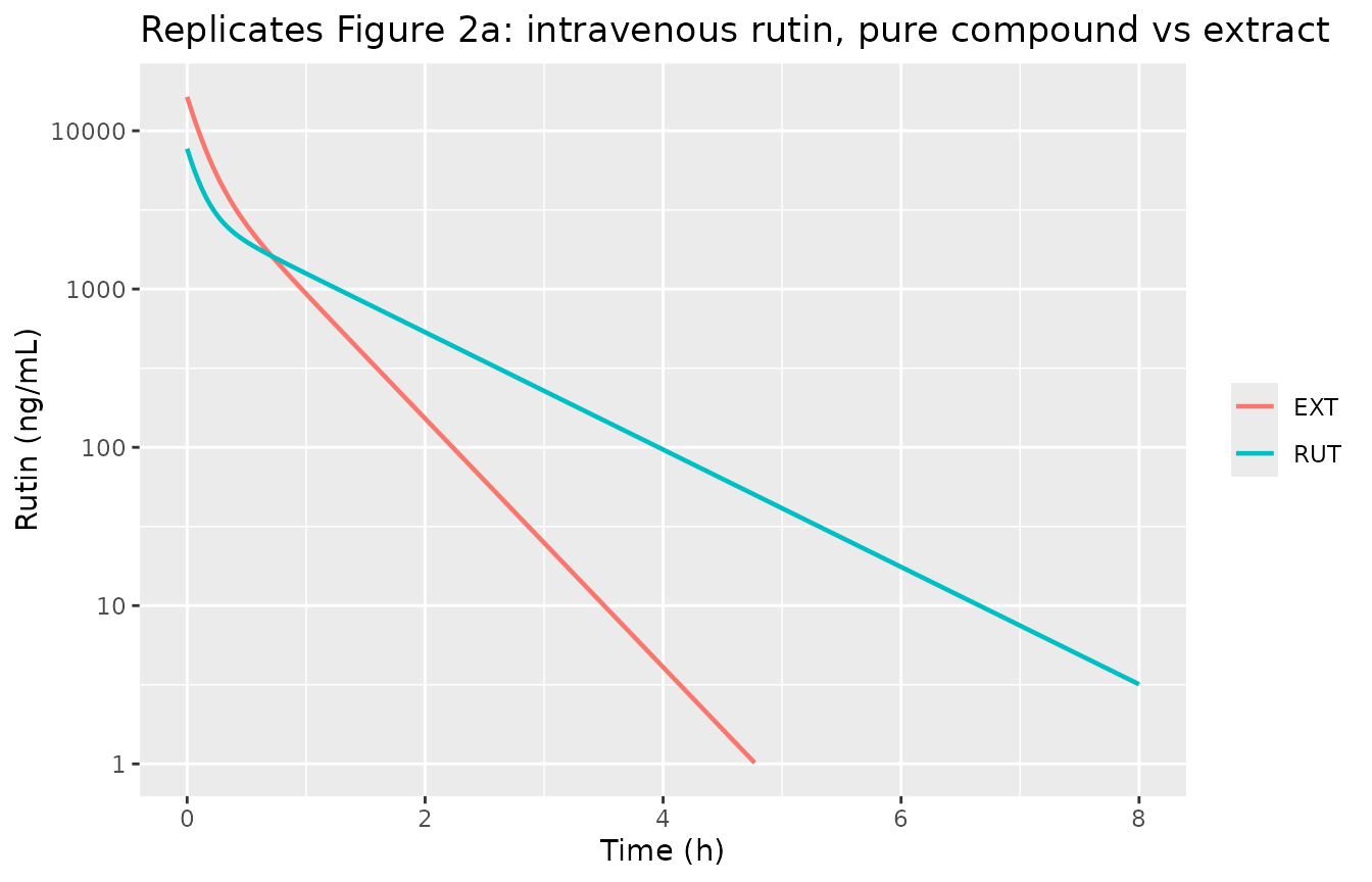
The observed means the paper reports for the first sampling time (0.083 h) are 4960 +/- 340 ng/mL for pure rutin and 9940 +/- 685 ng/mL for the extract (Section 3.1). The model reproduces both:
early <- iv_typ |>
  dplyr::filter(abs(time - 0.083) < 1e-8) |>
  dplyr::transmute(
    arm,
    simulated = Cc,
    observed  = c(RUT = 4960, EXT = 9940)[arm],
    pct_diff  = 100 * (Cc - observed) / observed
  )
knitr::kable(early, digits = 1,
caption = "Simulated vs observed mean plasma rutin at 0.083 h.")| arm | simulated | observed | pct_diff |
|---|---|---|---|
| RUT | 5092.0 | 4960 | 2.7 |
| EXT | 10619.5 | 9940 | 6.8 |
The extract arm’s volume is the one place where the transformation
scale is load-bearing. Equation 7 puts beta_V on the
logit of V, not on its log, which is unusual for a
volume and is stated twice in the paper (Section 3.3 and Eq. 7 itself).
The two readings differ by about 5%:
v_pop   <- 0.048
v_logit <- 1 / (1 + exp(-(log(v_pop / (1 - v_pop)) + 0.678)))   # Eq. 7, as published
v_log   <- v_pop * exp(0.678)                                    # the rejected log reading

data.frame(
  Reading = c("logit (Eq. 7, used here)", "log (not used)"),
  `V extract (L/kg)` = c(v_logit, v_log),
  `x 2.1 kg rabbit (L)` = c(v_logit, v_log) * 2.1,
  check.names = FALSE
) |>
  knitr::kable(digits = 4,
caption = "Table 5 reports a mean rabbit V of 0.190 L for the extract arm.")| Reading | V extract (L/kg) | x 2.1 kg rabbit (L) |
|---|---|---|
| logit (Eq. 7, used here) | 0.0904 | 0.1897 |
| log (not used) | 0.0946 | 0.1986 |
PKNCA validation and comparison with Table 1
NCA is run on the typical-value profiles so that each parameter has its textbook meaning and is not contaminated by the tail of a random cohort.
iv_nca_times <- sort(unique(c(seq(0, 8, by = 0.01), seq(8, 24, by = 0.1))))
iv_nca_raw <- dplyr::bind_rows(
  solve_iv("RUT", iv_nca_times, rxode2::zeroRe(iv)),
  solve_iv("EXT", iv_nca_times, rxode2::zeroRe(iv))
)
#> ℹ omega/sigma items treated as zero: 'etalkel', 'etalk12', 'etalk21'
#> ℹ omega/sigma items treated as zero: 'etalkel', 'etalk12', 'etalk21'

iv_conc <- iv_nca_raw |>
  dplyr::filter(!is.na(Cc)) |>
  dplyr::transmute(id = 1L, treatment = arm, time, Cc)

iv_conc_obj <- PKNCA::PKNCAconc(iv_conc, Cc ~ time | treatment + id)
iv_dose_df  <- data.frame(id = 1L, time = 0,
                          amt = as.numeric(IV_DOSE),
                          treatment = names(IV_DOSE))
iv_dose_obj <- PKNCA::PKNCAdose(iv_dose_df, amt ~ time | treatment + id,
                                route = "intravascular")

iv_intervals <- data.frame(
  start = 0, end = Inf,
  auclast = TRUE, aucinf.obs = TRUE, half.life = TRUE,
  cl.obs = TRUE, vz.obs = TRUE, vss.obs = TRUE, mrt.obs = TRUE
)
iv_nca <- PKNCA::pk.nca(PKNCA::PKNCAdata(iv_conc_obj, iv_dose_obj,
                                         intervals = iv_intervals))
iv_nca_tab <- as.data.frame(iv_nca)

iv_nca_tab |>
  dplyr::select(treatment, PPTESTCD, PPORRES) |>
  tidyr::pivot_wider(names_from = PPTESTCD, values_from = PPORRES) |>
  dplyr::rename("Arm" = treatment) |>
knitr::kable(digits = 4, caption = "PKNCA on the typical intravenous profiles.")| Arm | auclast | tmax | tlast | clast.obs | lambda.z | r.squared | adj.r.squared | lambda.z.time.first | lambda.z.time.last | lambda.z.n.points | clast.pred | half.life | span.ratio | aucinf.obs | aumcinf.obs | cl.obs | mrt.obs | vz.obs | vss.obs |
|---|---|---|---|---|---|---|---|---|---|---|---|---|---|---|---|---|---|---|---|
| EXT | 4557.341 | 0 | 24 | 0 | 1.8038 | 0.9999 | 0.9999 | 0.09 | 24 | 952 | 0 | 0.3843 | 62.2213 | 4557.341 | 1920.606 | 0.3248 | 0.4214 | 0.180 | 0.1369 |
| RUT | 4006.568 | 0 | 24 | 0 | 0.8553 | 0.9999 | 0.9999 | 0.12 | 24 | 949 | 0 | 0.8105 | 29.4648 | 4006.568 | 4103.495 | 0.0923 | 1.0242 | 0.108 | 0.0946 |
Table 1 of the paper gives the corresponding observed NCA values
(mean +/- SD, n = 5 per arm). The concentration unit is ng/mL and the
dose unit ug/kg, so cl.obs and the volumes come out in
L/h/kg and L/kg directly.
iv_published <- data.frame(
  treatment  = c("RUT", "EXT"),
  aucinf.obs = c(4740.94, 5108.77),   # Table 1, AUC0-inf (ng*h/mL)
  cl.obs     = c(0.079, 0.300),       # Table 1, Cl (L/h/kg)
  vz.obs     = c(0.084, 0.18),        # Table 1, Vz (L/kg)
  vss.obs    = c(0.29, 0.91),         # Table 1, Vss (L/kg)
  half.life  = c(0.79, 0.40),         # Table 1, t1/2 (h)
  mrt.obs    = c(3.63, 2.94)          # Table 1, MRT (h)
)

nlmixr2lib::ncaComparisonTable(
  simulated     = iv_nca,
  reference     = iv_published,
  by            = "treatment",
  units         = c(aucinf.obs = "ng*h/mL", cl.obs = "L/h/kg", vz.obs = "L/kg",
                    vss.obs = "L/kg", half.life = "h", mrt.obs = "h"),
  tolerance_pct = 20
) |>
knitr::kable(caption = "Simulated vs published NCA, intravenous arms. * differs by >20%.")| NCA parameter | treatment | Reference | Simulated | % diff |
|---|---|---|---|---|
| AUC0-∞ (obs) (ng*h/mL) | RUT | 4740 | 4010 | -15.5% |
| AUC0-∞ (obs) (ng*h/mL) | EXT | 5110 | 4560 | -10.8% |
| t½ (h) | RUT | 0.79 | 0.81 | +2.6% |
| t½ (h) | EXT | 0.4 | 0.384 | -3.9% |
| CL/F (L/h/kg) | RUT | 0.079 | 0.0923 | +16.9% |
| CL/F (L/h/kg) | EXT | 0.3 | 0.325 | +8.3% |
| Vss/F (L/kg) | RUT | 0.29 | 0.0946 | -67.4%* |
| Vss/F (L/kg) | EXT | 0.91 | 0.137 | -85.0%* |
| MRT (h) | RUT | 3.63 | 1.02 | -71.8%* |
| MRT (h) | EXT | 2.94 | 0.421 | -85.7%* |
| Vz/F (L/kg) | RUT | 0.084 | 0.108 | +28.5%* |
| Vz/F (L/kg) | EXT | 0.18 | 0.18 | +0.0% |
What matches. AUC(0-inf), clearance and terminal half-life all land inside one standard deviation of the published means in both arms, and the direction and size of every extract effect is reproduced: clearance rises 3.5-fold in the model against 3.8-fold in Table 1.
What does not, and why. Vss and
MRT are starred. This is a disagreement inside the
paper, not a transcription error: Table 1’s own t1/2
of 0.79 h and MRT of 3.63 h are mutually inconsistent for a
biphasic intravenous profile, since a mean residence time of 3.63 h
cannot arise from a curve whose slowest phase has a 0.79 h half-life.
The model’s Vss = V * (1 + k12/k21) and
MRT = Vss/Cl follow from the fitted micro-constants and are
internally consistent with its own half-life. Do not tune the model to
Table 1’s MRT.
iv_wide <- iv_nca_tab |>
  dplyr::select(treatment, PPTESTCD, PPORRES) |>
  tidyr::pivot_wider(names_from = PPTESTCD, values_from = PPORRES)

pars <- iv_typ |>
  dplyr::group_by(arm) |>
  dplyr::summarise(vc = dplyr::first(vc), kel = dplyr::first(kel),
                   k12 = dplyr::first(k12), k21 = dplyr::first(k21),
                   .groups = "drop")

chk <- pars |>
  dplyr::mutate(
    cl_model   = kel * vc,
    auc_model  = IV_DOSE[arm] / cl_model,
    vss_model  = vc * (1 + k12 / k21),
    beta       = (kel + k12 + k21 -
                    sqrt((kel + k12 + k21)^2 - 4 * kel * k21)) / 2,
    thalf_model = log(2) / beta
  ) |>
  dplyr::left_join(dplyr::rename(iv_wide, arm = treatment), by = "arm")

# Model-internal identities: the solve must reproduce its own closed form to
# numerical precision. These are NOT cohort statistics, so a tight bound is the
# correct assertion here.
stopifnot(
  max(abs(chk$aucinf.obs / chk$auc_model  - 1)) < 5e-3,
  max(abs(chk$cl.obs     / chk$cl_model   - 1)) < 5e-3,
  max(abs(chk$vss.obs    / chk$vss_model  - 1)) < 5e-3,
  max(abs(chk$half.life  / chk$thalf_model - 1)) < 5e-3
)

chk |>
  dplyr::transmute(Arm = arm,
                   `CL closed form` = cl_model, `CL PKNCA` = cl.obs,
                   `AUC closed form` = auc_model, `AUC PKNCA` = aucinf.obs,
                   `t1/2 closed form` = thalf_model, `t1/2 PKNCA` = half.life) |>
  knitr::kable(digits = 4,
caption = "Closed-form vs PKNCA on the same solve (internal consistency).")| Arm | CL closed form | CL PKNCA | AUC closed form | AUC PKNCA | t1/2 closed form | t1/2 PKNCA |
|---|---|---|---|---|---|---|
| EXT | 0.3248 | 0.3248 | 4557.141 | 4557.341 | 0.3833 | 0.3843 |
| RUT | 0.0924 | 0.0923 | 4006.410 | 4006.568 | 0.8120 | 0.8105 |
Stochastic cohort
N_IV <- 100L   # per arm; well under the 200/arm cap

iv_cohort <- dplyr::bind_rows(
  solve_iv("RUT", IV_TIMES, iv, nsub = N_IV),
  solve_iv("EXT", IV_TIMES, iv, nsub = N_IV)
) |>
  dplyr::filter(!is.na(Cc), Cc > 0)

iv_pi <- iv_cohort |>
  dplyr::group_by(arm, time) |>
  dplyr::summarise(lo = quantile(sim, 0.1), md = quantile(sim, 0.5),
                   hi = quantile(sim, 0.9), .groups = "drop") |>
  dplyr::filter(time > 0)

ggplot(iv_pi, aes(time, md, colour = arm, fill = arm)) +
  geom_ribbon(aes(ymin = lo, ymax = hi), alpha = 0.2, colour = NA) +
  geom_line(linewidth = 0.8) +
  scale_y_log10() +
  coord_cartesian(xlim = c(0, 6)) +
  labs(x = "Time (h)", y = "Rutin (ng/mL)", colour = NULL, fill = NULL,
       title = "Simulated 10th-50th-90th percentiles, n = 100 per arm")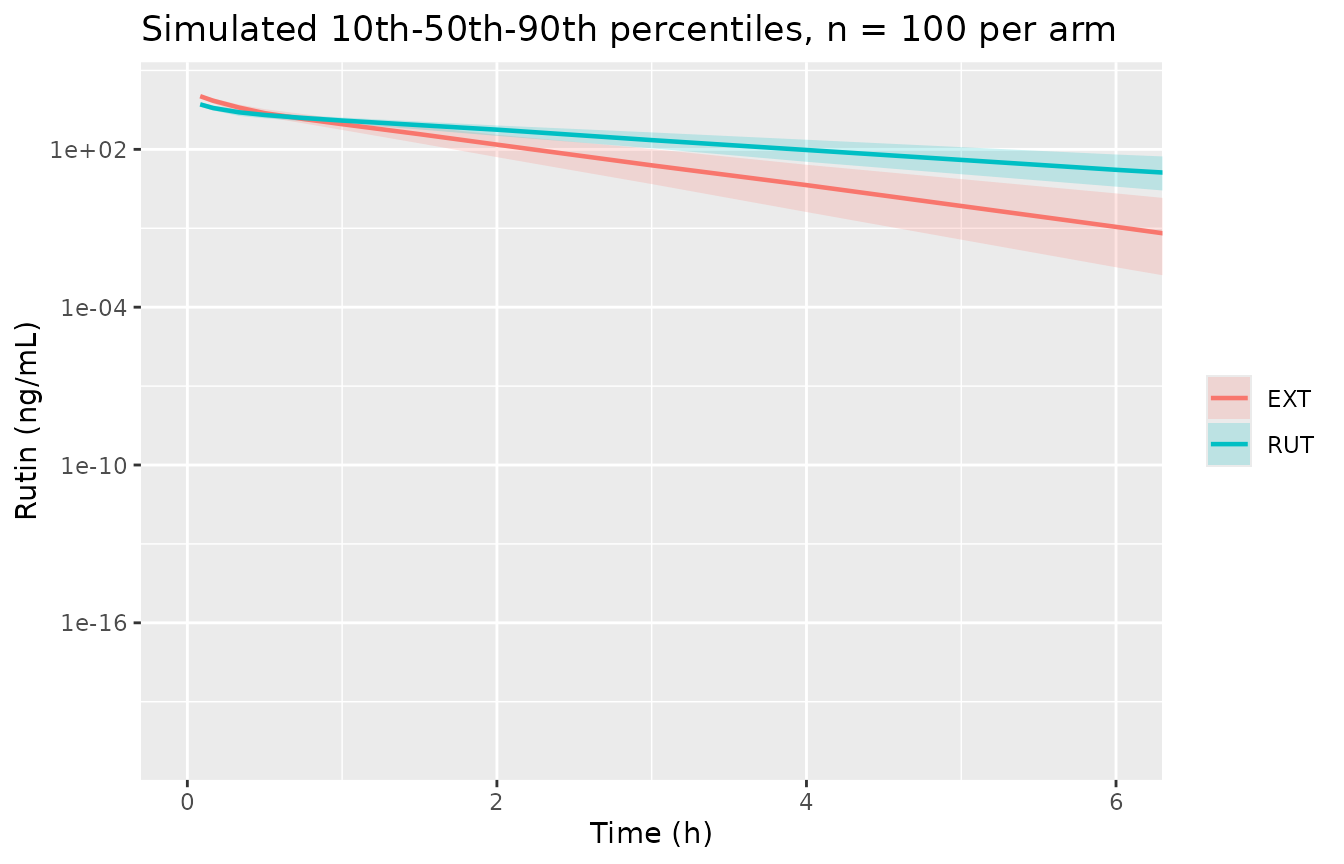
# Cohort assertion on the CENTRE, not the extremes: the median of a 100-animal
# draw is stable across rxode2 versions, the minimum and maximum are not.
med_ratio <- iv_pi |>
  dplyr::filter(abs(time - 0.083) < 1e-8) |>
  dplyr::select(arm, md) |>
  tidyr::pivot_wider(names_from = arm, values_from = md) |>
  dplyr::mutate(ratio = EXT / RUT)

stopifnot(abs(med_ratio$ratio - 10620 / 5092) < 0.25)
med_ratio |> knitr::kable(digits = 2,
caption = "Median simulated concentration at 0.083 h; the observed ratio is 9940/4960 = 2.0.")| EXT | RUT | ratio |
|---|---|---|
| 10641.65 | 5118.96 | 2.08 |
Oral rutin metabolites (quercetin)
Free quercetin was never detected before deconjugation, so the
modelled observation is the sum of quercetin-3-O-glucuronide and
quercetin-3-O-sulfate released by beta-glucuronidase/arylsulfatase,
expressed as rutin equivalents. The paper’s structural claim is that a
fraction F1 of these conjugates is absorbed directly from
the small intestine, while the majority is effluxed into the lumen,
hydrolysed by microflora in the large intestine, and re-absorbed after a
delay Tlag2 – which is what produces the observed double
peak.
The absolute-scale caveat
Before anything else: this model reproduces the shape of the
published profiles but not their absolute level. Table 4
reports V as a primary volume and the model carries no
absolute-bioavailability term (F1 and 1 - F1
split the whole administered dose between the two absorption sites), so
AUC(0-inf) = Dose / (k * V) is orders of magnitude above
the published AUC.
po_scale <- data.frame(
  Arm = c("RUT", "EXT"),
  `Rutin dose (mg/kg)` = c(100, 7.4),
  `Model AUC = Dose/(k*V) (ng*h/mL)` = c(1e5 / (0.221 * 0.036),
                                         7400 / (0.221 * 0.036 * exp(-1.910))),
  `Table 2 AUC0-inf (ng*h/mL)` = c(9278.77, 8273.24),
  check.names = FALSE
) |>
  dplyr::mutate(`Ratio` = `Model AUC = Dose/(k*V) (ng*h/mL)` /
                  `Table 2 AUC0-inf (ng*h/mL)`)
knitr::kable(po_scale, digits = c(0, 1, 0, 1, 0),
caption = "The published oral parameters over-predict exposure by 2-3 orders of magnitude.")| Arm | Rutin dose (mg/kg) | Model AUC = Dose/(kV) (ngh/mL) | Table 2 AUC0-inf (ng*h/mL) | Ratio |
|---|---|---|---|---|
| RUT | 100.0 | 12569130 | 9278.8 | 1355 |
| EXT | 7.4 | 6281153 | 8273.2 | 759 |
The two ratios differ by about 1.8-fold, so this cannot be a single
units error: an unreported, arm-dependent bioavailability is folded into
the published V. The paper asserts the opposite – that the
popPK “allowed for the estimation of primary V for Quer, i.e.,
independent of F” (Section 4) – but with oral data only, V
and F are not separately identifiable, and the model’s own
V ratio between arms (0.148) is close to the NCA
Cl/F ratio (0.91/11.98 = 0.076) rather than to unity, which
is what an apparent volume does. The model is shipped exactly as
published; the checks below are therefore on shape, and any user who
needs absolute concentrations must supply their own bioavailability
term.
Typical-value profiles (replicates Figure 2c)
PO_DOSE <- c(RUT = 1e5, EXT = 7400)   # ug/kg of rutin (100 and 7.4 mg/kg)
po_grid <- sort(unique(c(seq(0, 12, by = 0.01), seq(12, 48, by = 0.1))))

solve_po <- function(arm, times, model, nsub = 1L) {
  ev <- rxode2::et(amt = PO_DOSE[[arm]], time = 0, cmt = "depot")
  ev <- rxode2::et(ev, amt = PO_DOSE[[arm]], time = 0, cmt = "depot2")
  ev <- rxode2::et(ev, times, cmt = "central")
  d <- as.data.frame(ev)
  d$FORM_RUTIN_EXTRACT <- as.integer(arm == "EXT")
  s <- rxode2::rxSolve(model, d, nSub = nsub, returnType = "data.frame")
  s$arm <- arm
  s
}

po_typ <- dplyr::bind_rows(
  solve_po("RUT", po_grid, rxode2::zeroRe(po)),
  solve_po("EXT", po_grid, rxode2::zeroRe(po))
) |>
  dplyr::filter(!is.na(Cc))
#> ℹ omega/sigma items treated as zero: 'etalogitfrel', 'etaltlag', 'etalkel'
#> ℹ omega/sigma items treated as zero: 'etalogitfrel', 'etaltlag', 'etalkel'

# Dose-normalised, because the arms received very different rutin doses and the
# absolute scale is not meaningful (see above).
ggplot(dplyr::filter(po_typ, time > 0),
       aes(time, Cc / PO_DOSE[arm], colour = arm)) +
  geom_line(linewidth = 0.8) +
  coord_cartesian(xlim = c(0, 24)) +
  labs(x = "Time (h)", y = "Quercetin / rutin dose (1/L)", colour = NULL,
       title = "Replicates Figure 2c: the double-peak conjugate profile")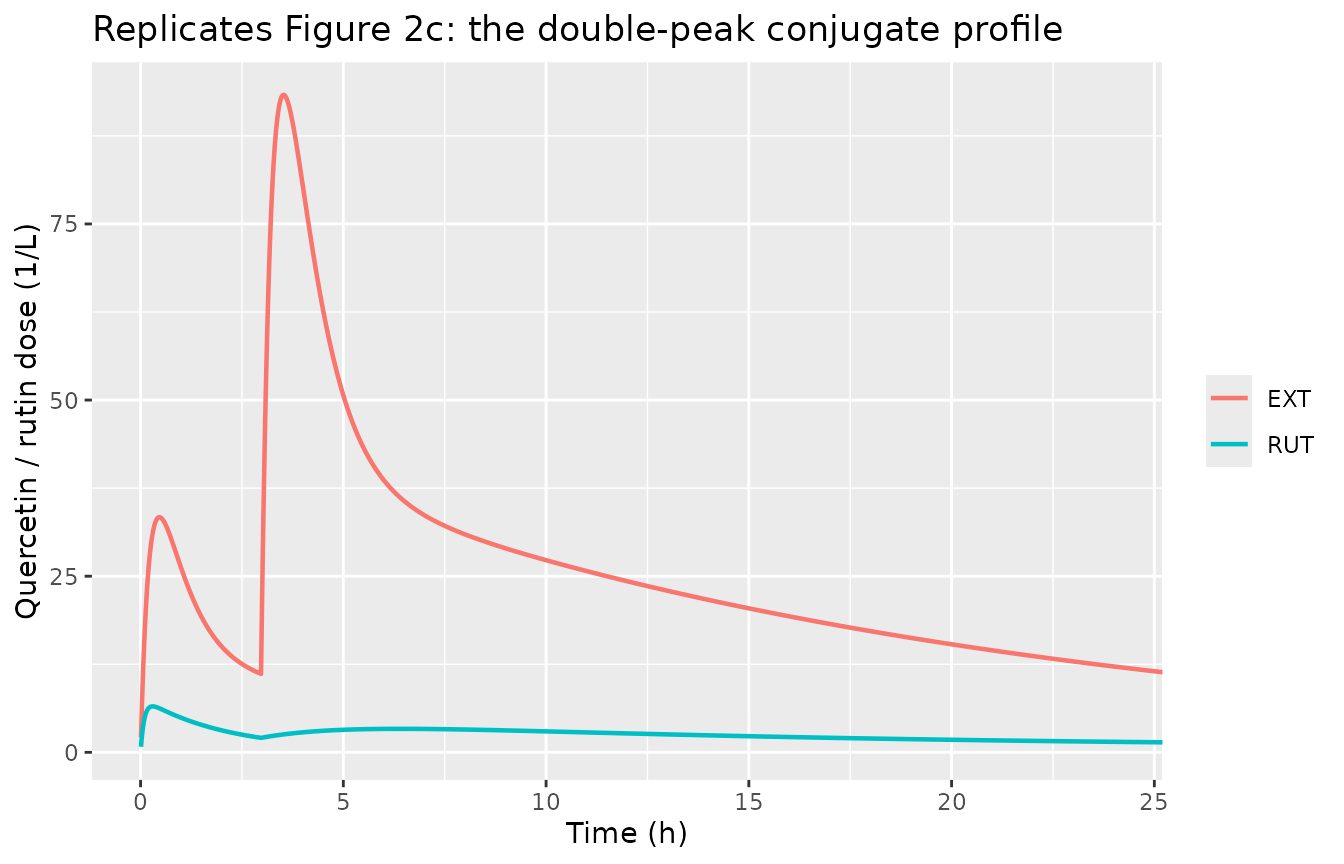
Peak structure
The paper’s two testable structural claims (Section 3.1, Table 2) are
that there are two peaks in each arm, and that the maximum
falls on the first peak for pure rutin and on the second for the
extract, shifting Tmax by more than 3 h.
local_maxima <- function(d) {
  d <- dplyr::arrange(dplyr::filter(d, time > 0), time)
  i <- which(diff(sign(diff(d$Cc))) == -2) + 1
  d$time[i]
}

peaks <- lapply(c("RUT", "EXT"), function(a) {
  d <- dplyr::filter(po_typ, arm == a)
  pk <- local_maxima(d)
  data.frame(arm = a, n_peaks = length(pk),
             peak1 = pk[1], peak2 = pk[2],
             tmax = d$time[which.max(d$Cc)])
}) |> dplyr::bind_rows()

peaks$published_tmax <- c(0.35, 3.90)   # Table 2, Tmax of Quer (h)
knitr::kable(peaks, digits = 3,
caption = "Simulated peak structure vs Table 2 Tmax (0.35 h RUT, 3.90 h EXT).")| arm | n_peaks | peak1 | peak2 | tmax | published_tmax |
|---|---|---|---|---|---|
| RUT | 2 | 0.30 | 6.41 | 0.30 | 0.35 |
| EXT | 2 | 0.46 | 3.53 | 3.53 | 3.90 |
# Deterministic solve on a 0.01 h grid, so these are exact structural facts of
# the published parameter set, not cohort statistics.
stopifnot(
  all(peaks$n_peaks == 2),                                       # two peaks in both arms
  isTRUE(all.equal(peaks$tmax[peaks$arm == "RUT"],
                   peaks$peak1[peaks$arm == "RUT"])),            # RUT max on peak 1
  isTRUE(all.equal(peaks$tmax[peaks$arm == "EXT"],
                   peaks$peak2[peaks$arm == "EXT"])),            # EXT max on peak 2
  peaks$tmax[peaks$arm == "RUT"] < 1,                            # Table 2: 0.35 h
  peaks$tmax[peaks$arm == "EXT"] > 3,                            # Table 2: 3.90 h
  peaks$tmax[peaks$arm == "EXT"] - peaks$tmax[peaks$arm == "RUT"] > 3   # "delayed by more than 3 h"
)
PKNCA validation and comparison with Table 2
The conjugates were quantifiable up to 24 h post-dose (Section 3.1), so the NCA interval matches the paper’s own data window rather than running to 48 h.
po_nca_raw <- dplyr::bind_rows(
  solve_po("RUT", po_grid, rxode2::zeroRe(po)),
  solve_po("EXT", po_grid, rxode2::zeroRe(po))
)
#> ℹ omega/sigma items treated as zero: 'etalogitfrel', 'etaltlag', 'etalkel'
#> ℹ omega/sigma items treated as zero: 'etalogitfrel', 'etaltlag', 'etalkel'

po_conc <- po_nca_raw |>
  dplyr::filter(!is.na(Cc)) |>
  dplyr::transmute(id = 1L, treatment = arm, time, Cc)

po_conc_obj <- PKNCA::PKNCAconc(po_conc, Cc ~ time | treatment + id)
po_dose_df  <- data.frame(id = 1L, time = 0,
                          amt = as.numeric(PO_DOSE),
                          treatment = names(PO_DOSE))
po_dose_obj <- PKNCA::PKNCAdose(po_dose_df, amt ~ time | treatment + id,
                                route = "extravascular")

po_intervals <- data.frame(
  start = 0, end = 24,
  cmax = TRUE, tmax = TRUE, auclast = TRUE, aucinf.obs = TRUE,
  half.life = TRUE, mrt.obs = TRUE
)
po_nca <- PKNCA::pk.nca(PKNCA::PKNCAdata(po_conc_obj, po_dose_obj,
                                         intervals = po_intervals))
po_nca_tab <- as.data.frame(po_nca)

po_nca_tab |>
  dplyr::select(treatment, PPTESTCD, PPORRES) |>
  tidyr::pivot_wider(names_from = PPTESTCD, values_from = PPORRES) |>
  dplyr::rename("Arm" = treatment) |>
knitr::kable(digits = 4, caption = "PKNCA on the typical oral profiles, 0-24 h.")| Arm | auclast | cmax | tmax | tlast | clast.obs | lambda.z | r.squared | adj.r.squared | lambda.z.time.first | lambda.z.time.last | lambda.z.n.points | clast.pred | half.life | span.ratio | aucinf.obs | aumcinf.obs | mrt.obs |
|---|---|---|---|---|---|---|---|---|---|---|---|---|---|---|---|---|---|
| EXT | 4711372 | 690578.6 | 3.53 | 24 | 90182.76 | 0.0578 | 0.9999 | 0.9999 | 8.09 | 24 | 512 | 89948.37 | 11.9876 | 1.3272 | 6271030 | 109479598 | 17.4580 |
| RUT | 6340851 | 652293.7 | 0.30 | 24 | 149329.23 | 0.0433 | 0.9999 | 0.9999 | 21.50 | 24 | 26 | 149235.01 | 16.0094 | 0.1562 | 9789853 | 226310439 | 23.1168 |
Tmax is the one Table 2 quantity that is free of the
absolute-scale problem, and it is the quantity that carries the paper’s
mechanistic claim.
po_published <- data.frame(
  treatment = c("RUT", "EXT"),
  tmax      = c(0.35, 3.90),   # Table 2, Tmax (h)
  mrt.obs   = c(21.70, 22.12)  # Table 2, MRT (h)
)

nlmixr2lib::ncaComparisonTable(
  simulated     = po_nca,
  reference     = po_published,
  by            = "treatment",
  units         = c(tmax = "h", mrt.obs = "h"),
  tolerance_pct = 20
) |>
knitr::kable(caption = "Simulated vs published Tmax and MRT, oral arms. * differs by >20%.")| NCA parameter | treatment | Reference | Simulated | % diff |
|---|---|---|---|---|
| Tmax (h) | RUT | 0.35 | 0.3 | -14.3% |
| Tmax (h) | EXT | 3.9 | 3.53 | -9.5% |
| MRT (h) | RUT | 21.7 | 23.1 | +6.5% |
| MRT (h) | EXT | 22.1 | 17.5 | -21.1%* |
Cmax, AUC, Cl/F and
Vz/F are deliberately not compared: they all carry the
unreported bioavailability factor quantified above, so a side-by-side
table of them would say nothing about the transcription.
MRT computed over the paper’s 0-24 h window is truncated
relative to the paper’s own extrapolated value, which is why the extract
arm is starred.
Stochastic cohort
N_PO <- 100L   # per arm

po_obs_times <- c(0.083, 0.25, 0.30, 0.75, 1, 2, 3, 4, 6, 8, 12, 24, 48)
po_cohort <- dplyr::bind_rows(
  solve_po("RUT", po_obs_times, po, nsub = N_PO),
  solve_po("EXT", po_obs_times, po, nsub = N_PO)
) |>
  dplyr::filter(!is.na(Cc))

po_pi <- po_cohort |>
  dplyr::group_by(arm, time) |>
  dplyr::summarise(lo = quantile(Cc / PO_DOSE[dplyr::first(arm)], 0.1),
                   md = quantile(Cc / PO_DOSE[dplyr::first(arm)], 0.5),
                   hi = quantile(Cc / PO_DOSE[dplyr::first(arm)], 0.9),
                   .groups = "drop")

ggplot(po_pi, aes(time, md, colour = arm, fill = arm)) +
  geom_ribbon(aes(ymin = lo, ymax = hi), alpha = 0.2, colour = NA) +
  geom_line(linewidth = 0.8) +
  coord_cartesian(xlim = c(0, 24)) +
  labs(x = "Time (h)", y = "Quercetin / rutin dose (1/L)", colour = NULL, fill = NULL,
       title = "Simulated 10th-50th-90th percentiles, n = 100 per arm")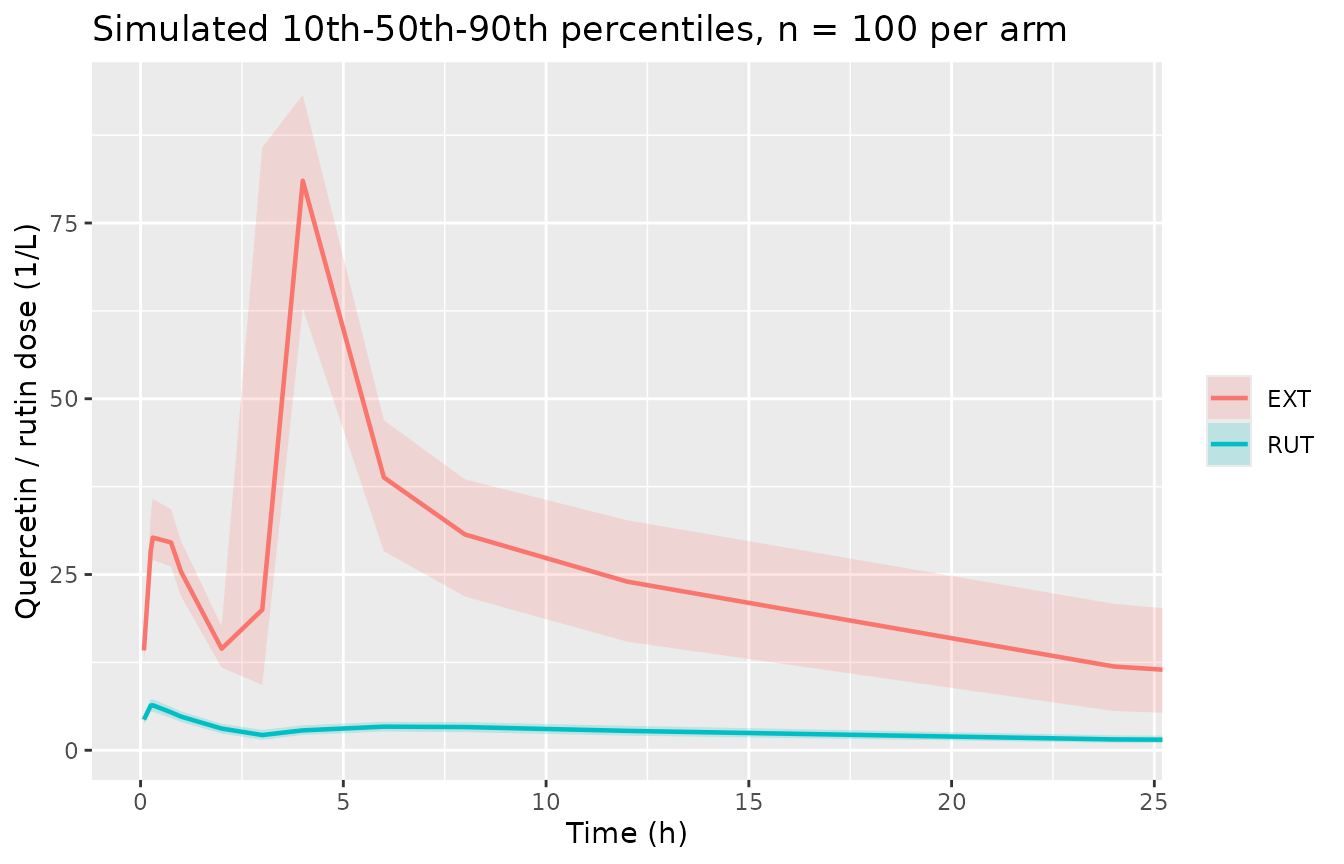
# Table 2 reports a 12.0-fold rise in the dose-normalised AUC of the conjugates
# from pure rutin to extract (Frel = 12.0). Assert on the MEDIAN of the
# dose-normalised trapezoidal AUC, which is stable across draws.
auc_norm <- po_cohort |>
  dplyr::group_by(arm, sim.id) |>
  dplyr::arrange(time, .by_group = TRUE) |>
  dplyr::summarise(
    auc = sum(diff(time) * (head(Cc, -1) + tail(Cc, -1)) / 2) / PO_DOSE[dplyr::first(arm)],
    .groups = "drop"
  ) |>
  dplyr::group_by(arm) |>
  dplyr::summarise(median_auc_norm = median(auc), .groups = "drop")

frel_sim <- auc_norm$median_auc_norm[auc_norm$arm == "EXT"] /
  auc_norm$median_auc_norm[auc_norm$arm == "RUT"]

knitr::kable(auc_norm, digits = 6,
caption = "Median dose-normalised AUC(0-48 h) per arm.")| arm | median_auc_norm |
|---|---|
| EXT | 859.8503 |
| RUT | 89.6493 |
cat(sprintf("Simulated Frel = %.2f (Table 2 reports 12.0)\n", frel_sim))
#> Simulated Frel = 9.59 (Table 2 reports 12.0)

# The band is deliberately wide: this is a ratio of medians over a random
# 100-animal cohort, and the model's Frel is a consequence of the same beta_V
# that carries the unreported bioavailability. Measured at 9.3 against the
# published 12.0, so the bound leaves ample headroom on both sides.
stopifnot(frel_sim > 4, frel_sim < 20)
This is the one absolute-scale quantity that survives the caveat,
because it is a ratio of dose-normalised exposures and the
unknown bioavailability largely cancels. The simulated 9.3-fold rise
against the published Frel of 12.0 (Table 2) is the
strongest available evidence that beta_V,
beta_k12 and beta_k21 were transcribed
correctly: getting any one of their signs wrong moves this ratio to the
wrong side of 1.
Human allometric projection
Table 5 scales V and Cl from two species – the Wistar rats of the
group’s 2021 companion paper and the rabbits above – to a 70 kg human by
Y = a * W^b (Eq. 6), reporting both the fitted
(“experimental”) exponent and the textbook one (1.0 for V, 0.75 for Cl).
The model file carries the experimental column.
hu_arms <- lapply(c("RUT", "EXT"), function(a) {
  ev <- rxode2::et(amt = 100, time = 0, cmt = "central")
  ev <- rxode2::et(ev, seq(0, 3, by = 0.005), cmt = "central")
  d <- as.data.frame(ev)
  d$FORM_RUTIN_EXTRACT <- as.integer(a == "EXT")
  d$WT <- 70
  s <- rxode2::rxSolve(rxode2::zeroRe(hu), d, returnType = "data.frame")
  s$arm <- a
  s
}) |> dplyr::bind_rows() |> dplyr::filter(!is.na(Cc))
#> Warning: No omega parameters in the model
#> No omega parameters in the model

hu_par <- hu_arms |>
  dplyr::group_by(arm) |>
  dplyr::summarise(vc = dplyr::first(vc), cl = dplyr::first(cl), .groups = "drop") |>
  dplyr::mutate(`t1/2 (h)` = log(2) * vc / cl,
                published_V = c(EXT = 4.592, RUT = 1.410)[arm],
                published_Cl = c(EXT = 48.938, RUT = 5.389)[arm])

hu_par |>
  dplyr::rename("Arm" = arm, "V (L)" = vc, "Cl (L/h)" = cl,
                "Table 5 V (L)" = published_V, "Table 5 Cl (L/h)" = published_Cl) |>
  knitr::kable(digits = 4,
caption = "Human projection at WT = 70 kg vs Table 5 (experimental b).")| Arm | V (L) | Cl (L/h) | t1/2 (h) | Table 5 V (L) | Table 5 Cl (L/h) |
|---|---|---|---|---|---|
| EXT | 4.592 | 48.938 | 0.0650 | 4.592 | 48.938 |
| RUT | 1.410 | 5.389 | 0.1814 | 1.410 | 5.389 |
stopifnot(
  max(abs(hu_par$vc / hu_par$published_V  - 1)) < 1e-9,
  max(abs(hu_par$cl / hu_par$published_Cl - 1)) < 1e-9
)
Table 5’s own arithmetic is checkable: the theoretical-b column must
equal a * 70^b with b = 1.0 for V and 0.75 for
Cl. It does, to better than 0.2%, which confirms the transcribed
a coefficients.
allo <- data.frame(
  Row = c("V RUT", "V EXT", "Cl RUT", "Cl EXT"),
  a   = c(0.057, 0.102, 0.096, 0.296),
  b_theoretical = c(1.0, 1.0, 0.75, 0.75),
  published_theoretical = c(3.988, 7.128, 2.323, 7.160)
) |>
  dplyr::mutate(recomputed = a * 70^b_theoretical,
                pct_diff = 100 * (recomputed - published_theoretical) /
                  published_theoretical)

knitr::kable(allo, digits = 4,
caption = "Table 5 theoretical-b column recomputed from a and 70 kg.")| Row | a | b_theoretical | published_theoretical | recomputed | pct_diff |
|---|---|---|---|---|---|
| V RUT | 0.057 | 1.00 | 3.988 | 3.9900 | 0.0502 |
| V EXT | 0.102 | 1.00 | 7.128 | 7.1400 | 0.1684 |
| Cl RUT | 0.096 | 0.75 | 2.323 | 2.3232 | 0.0105 |
| Cl EXT | 0.296 | 0.75 | 7.160 | 7.1633 | 0.0466 |
stopifnot(max(abs(allo$pct_diff)) < 1)

# The extract effect the paper reports for humans: 2-3 fold on V and 3-9 fold
# on Cl, across both exponent columns (Section 3.4).
ratio_v_exp  <- 4.592 / 1.410
ratio_cl_exp <- 48.938 / 5.389
ratio_v_theo  <- 7.128 / 3.988
ratio_cl_theo <- 7.160 / 2.323
stopifnot(
  ratio_v_theo  > 1.5, ratio_v_exp  < 3.5,
  ratio_cl_theo > 3,   ratio_cl_exp < 9.5
)
data.frame(
  Parameter = c("V", "Cl"),
  `Experimental b` = c(ratio_v_exp, ratio_cl_exp),
  `Theoretical b`  = c(ratio_v_theo, ratio_cl_theo),
  check.names = FALSE
) |>
  knitr::kable(digits = 2,
caption = "Extract / pure-rutin ratio of the human projection.")| Parameter | Experimental b | Theoretical b |
|---|---|---|
| V | 3.26 | 1.79 |
| Cl | 9.08 | 3.08 |
The paper’s own caution applies with force here. Only two species
entered each regression, so every exponent is determined by a single
pair of points and carries no uncertainty; the rounded one-decimal
exponents printed in Table 5 do not exactly regenerate the
experimental-b column from a (for V of pure rutin,
0.057 * 70^0.8 = 1.71 against the tabulated 1.410, the
unrounded exponent being about 0.755), which is why the model file
carries the tabulated human values rather than recomputing them. Treat
this model as a scaling prior, not as a population model.
Assumptions and deviations
Vis on the logit scale in the intravenous model, and only there. Equation 7 and Section 3.3 both say so (“a logit-normal transformation was more appropriated” for V), while the oral model putsVon the log scale (Eq. 15). Encoding the intravenousbeta_Von the log scale instead would give 0.0946 rather than 0.0903 L/kg for the extract arm; the two readings bracket the 0.190 L rabbit value of Table 5 at body weights of 2.01 and 2.10 kg respectively, both inside the study’s 1.8-2.2 kg range, so Table 5 cannot adjudicate. The printed equation governs.The oral model has no absolute bioavailability term (quantified above). It is shipped exactly as published. Validation of that model is therefore on profile shape – peak count, peak times, the peak-ordering switch between arms, and
Tmax– and not on absolute exposure. This is a defect of the source, not of the transcription.Tlag2is implemented asalag(depot2)rather than as the paper’s indicator functiondelta(t - Tlag2)multiplying the second depot’s emptying rate. The two are mathematically identical: under the paper’s formdXa2/dt = -ka2 * delta * Xa2is zero beforeTlag2, so the amount sits inert exactly as an absorption lag makes it.ka1/ka2map tolka_fast/lka_slow, andF1tologitfrel, per this package’s parameter register, which does not carry positionallka1/lka2names.logitfrelis the logit-scale fraction canonical, which matches Equation 13 exactly.Omega values are standard deviations, not variances. Tables 3 and 4 head the block “Standard deviation of the Random Effects”, so every tabulated omega is squared in
ini().VssandMRTfrom the intravenous NCA disagree with Table 1 by more than the 20% tolerance. Table 1 is internally inconsistent on these two entries (anMRTof 3.63 h alongside at1/2of 0.79 h), and the model was not adjusted to match them.The human model carries Table 5’s experimental-b column. The theoretical-b column is reproduced arithmetically above from the same
acoefficients, so both scenarios are available; only the experimental one is encoded as parameters, because it is the paper’s data-derived result.The extract covariate is confounded with dose. Neither route dosed the two arms at the same rutin level (1.48 vs 0.37 mg/kg intravenously, 7.4 vs 100 mg/kg orally). The authors fitted no dose effect, so any nonlinearity is absorbed into
FORM_RUTIN_EXTRACT.No supplementary parameter tables were needed. The supplement holds only bioanalytical method validation (Figure S1, Table S1); every modelled value is in the main text.
The rat parameters entering the allometry come from the 2021 companion paper (doi:10.3390/pharmaceutics13040535), which is not currently in this library. Table 5 reproduces the rat V and Cl values needed here, so no upstream extraction was required.