Tacrolimus whole-blood and intracellular PBMC (Franken 2022)
Source:vignettes/articles/Franken_2022_tacrolimus.Rmd
Franken_2022_tacrolimus.RmdModel and source
- Citation: Franken LG, Francke MI, Andrews LM, van Schaik RHN, Li Y, de Wit LEA, Baan CC, Hesselink DA, de Winter BCM. A Population Pharmacokinetic Model of Whole-Blood and Intracellular Tacrolimus in Kidney Transplant Recipients. Eur J Drug Metab Pharmacokinet. 2022;47(4):523-535. doi:10.1007/s13318-022-00767-8. Whole-blood layer from: Andrews LM, Hesselink DA, van Schaik RHN, et al. A population pharmacokinetic model to predict the individual starting dose of tacrolimus in adult renal transplant recipients. Br J Clin Pharmacol. 2019;85(3):601-615. doi:10.1111/bcp.13838
- Description: Two-compartment population PK model with first-order absorption and an absorption lag time for twice-daily oral immediate-release tacrolimus (Prograft) in adult kidney transplant recipients, extended with an intracellular peripheral blood mononuclear cell (PBMC) effect compartment (Franken 2022 final model). The whole-blood layer is the Andrews 2019 model, carried unchanged: apparent oral clearance CL/F depends on CYP3A5 expresser status, CYP3A4*22 carriage, haematocrit, serum creatinine, serum albumin, age and body surface area, and apparent central volume V1/F on lean body mass. The PBMC compartment has no mass transfer from the central compartment: the intracellular concentration equilibrates with the whole-blood concentration at a fixed rate constant (0.9 1/h) towards a steady state 14.1-fold higher than whole blood, and this ratio rises with lean body mass (power exponent 1.01, centred at 59.5 kg) and falls with haematocrit (power exponent -1.22, centred at 34 percent), with 38.9 percent inter-individual variability. Residual error is proportional for whole blood and combined additive plus proportional for the PBMC concentration.
- Article: https://doi.org/10.1007/s13318-022-00767-8 (open access; the Electronic Supplementary Material holds Supplementary Table S1 and the NONMEM control stream, Supplementary Data S1)
Franken et al. extended the Andrews 2019 whole-blood tacrolimus model
(modellib("Andrews_2019_tacrolimus")) with a compartment
for the concentration inside peripheral blood mononuclear cells (PBMCs).
Each patient contributed a single pre-dose PBMC sample, so the
intracellular compartment was written as an effect compartment without
mass transfer (Figure 1, Equation 3):
The equilibration rate constant
could not be estimated from trough samples and was fixed at 0.9 1/h. The
steady-state ratio
(here ppc, the canonical effect-compartment
pseudo-partition coefficient) was estimated with a power effect of lean
body weight and of haematocrit (Equation 4).
Population
The model was developed from 590 tacrolimus concentrations (406 whole-blood, 184 intracellular) in 184 adult kidney transplant recipients from Erasmus MC, Rotterdam. All were participants in a randomized trial of CYP3A5 genotype-based versus body-weight-based tacrolimus dosing after living-donor transplantation (Shuker 2016). They received oral twice-daily Prograft with mycophenolic acid, prednisolone and basiliximab induction. Whole-blood pre-dose targets were 10-15 ng/mL in weeks 1-2, 8-12 ng/mL in weeks 3-4 and 5-10 ng/mL afterwards. Median age was 57 years (IQR 46-64), body weight 80.0 kg (69.2-92.0), lean body weight 60.9 kg (53.8-66.9) and haematocrit 0.34 L/L (0.31-0.38) (Table 1). 22.3% were CYP3A5 expressers and 10.9% carried CYP3A4*22. Table 1 reports neither sex nor race.
The same information is available programmatically via
readModelDb("Franken_2022_tacrolimus")()$population.
Source trace
Every whole-blood value is the Andrews 2019 estimate. Franken 2022 held these at their published values (Table 2 footnote a) and estimated only the intracellular parameters and the residual errors.
| Equation / parameter | Value | Source location |
|---|---|---|
ltlag |
log(0.38) h, fixed | Table 2 ‘T lag’; Data S1 ALAG1 = 0.382
|
lka |
log(3.58) 1/h, fixed | Table 2 ‘k a’; Data S1 KA = 3.6
|
lcl |
log(23.0) L/h, fixed | Table 2 ‘CL/F’ |
lvc |
log(692) L, fixed | Table 2 ‘V 1 /F’ |
lq |
log(11.6) L/h, fixed | Table 2 ‘Q 1 /F’ |
lvp |
log(5340) L, fixed | Table 2 ‘V 2 /F’ |
e_cyp3a5_expr_cl, e_cyp3a4_22_cl
|
1.63, 0.80, fixed | Table 2 ‘Covariate effect on CL’ |
e_hct_cl, e_creat_cl,
e_alb_cl, e_age_cl, e_bsa_cl
|
-0.76, -0.14, 0.43, -0.43, 0.88, fixed | Table 2 ‘Covariate effect on CL’ |
e_lbm_vc |
1.52, fixed | Table 2 ‘Covariate effect on V 1’ |
| CL/F and V1/F centring values (55.72 y, 42 g/L, 1.93 m^2, 134.98 umol/L, 34 %, 58.94 kg) | n/a | Andrews 2019 Data S1, as in
Andrews_2019_tacrolimus
|
etalcl, etalvc, etalvp,
etalq
|
38.6, 49.2, 53.0, 78.7 %CV, fixed | Table 2 ‘IIV’ |
lke0 |
log(0.9) 1/h, fixed | Table 2 ‘K WB-IC’; Results 3.2; Data S1 THETA(4)
|
lppc |
log(14100 / 1000) | Table 2 ‘R WB:IC’ final model; Equation 4; Data S1
THETA(5)
|
e_lbm_ppc |
1.01 | Table 2 ‘Covariate effect on R WB:IC’; Equation 4 |
e_hct_ppc |
-1.22 | Table 2; Equation 4 |
etalppc |
38.9 %CV -> 0.140910 | Table 2 ‘IIV R WB-IC’ |
propSd |
0.611 | Table 2 ‘Proportional WB’; Data S1 THETA(1)
|
propSd_Cpbmc, addSd_Cpbmc
|
0.184, 36.8 ng/mL | Table 2 ‘Proportional IC’, ‘Additive IC’; Data S1
THETA(2), THETA(3)
|
d/dt(effect) |
n/a | Equation 3; Data S1
DADT(4) = K24*(RPIC*(A(2)/V2)-A(4))
|
ppc covariate model |
n/a | Equation 4; Data S1
RPIC = THETA(5)*(LBW/59.5)**THETA(6)*(HCT/0.34)**THETA(7)
|
Cc <- central / vc * 1000 |
n/a | Data S1 S2 = V2 / 1000
|
| Residual error | n/a | Data S1 $ERROR (CMT 2 proportional; CMT 4 additive +
proportional; $SIGMA 1 FIX) |
Simulated subjects
Section 3.5 and Figure 4 simulate steady-state pre-dose concentrations for the 10th, 50th and 90th percentiles of one covariate, with the others at the population median. The haematocrit scenarios are 0.28, 0.34 and 0.43 L/L. The body-composition scenarios vary total body weight (58.5, 78.9 and 102 kg), which moves lean body weight (49.96, 60.62, 68.47 kg) and body surface area (1.68, 1.96, 2.22 m^2) together. Those six numbers are reproduced exactly by the paper’s own James and Mosteller formulas for a male patient 174.5 cm tall, so that is the simulated patient. The remaining covariates are the Table 1 medians: age 57 years, albumin 43 g/L, creatinine 135 umol/L. The patient is a CYP3A5 non-expresser without CYP3A4*22.
height_cm <- 174.5
lbm_james_male <- function(wt, ht) 1.1 * wt - 128 * (wt / ht)^2
bsa_mosteller <- function(wt, ht) sqrt(ht * wt / 3600)

scenarios <- tibble::tribble(
  ~panel, ~scenario, ~WT, ~HCT,
  "A: haematocrit", "Haematocrit 0.28 L/L", 78.9, 28,
  "A: haematocrit", "Haematocrit 0.34 L/L", 78.9, 34,
  "A: haematocrit", "Haematocrit 0.43 L/L", 78.9, 43,
  "B: body composition", "Weight 58.5 kg", 58.5, 34,
  "B: body composition", "Weight 78.9 kg", 78.9, 34,
  "B: body composition", "Weight 102 kg", 102, 34
) |>
  mutate(
    LBM = lbm_james_male(WT, height_cm),
    BSA = bsa_mosteller(WT, height_cm),
    AGE = 57, ALB = 43, CREAT = 135,
    CYP3A5_EXPR = 0, SNP_CYP3A4_RS35599367 = 0,
    scenario = factor(scenario, levels = scenario)
  )

# Figure 4B prints LBW 49.96 / 60.62 / 68.47 kg and BSA 1.68 / 1.96 / 2.22 m^2.
stopifnot(
  max(abs(scenarios$LBM[4:6] - c(49.96, 60.62, 68.47))) < 0.02,
  max(abs(scenarios$BSA[4:6] - c(1.68, 1.96, 2.22))) < 0.006
)
knitr::kable(scenarios[, c("scenario", "WT", "LBM", "BSA", "HCT")], digits = 2,
caption = "Simulated covariate scenarios (HCT in percent).")| scenario | WT | LBM | BSA | HCT |
|---|---|---|---|---|
| Haematocrit 0.28 L/L | 78.9 | 60.62 | 1.96 | 28 |
| Haematocrit 0.34 L/L | 78.9 | 60.62 | 1.96 | 34 |
| Haematocrit 0.43 L/L | 78.9 | 60.62 | 1.96 | 43 |
| Weight 58.5 kg | 58.5 | 49.96 | 1.68 | 34 |
| Weight 78.9 kg | 78.9 | 60.62 | 1.96 | 34 |
| Weight 102 kg | 102.0 | 68.47 | 2.22 | 34 |
The paper does not state the simulated dose. Every comparison below is either a ratio (the whole-blood:intracellular ratio does not depend on dose) or is normalised to the median scenario. A dose of 4 mg twice daily is used throughout.
dose <- 4
tau <- 12

# Two dosing schemes.
# * n_doses = NULL: the true periodic steady state, via ss = 1 on the first
#   dose. The 5340 L peripheral volume gives a slow terminal phase, so a dose
#   train would need months to get there. `grid` is time after that dose.
# * n_doses = k: k doses every tau from time 0, with one pre-dose observation
#   at k * tau, immediately before dose k + 1.
make_events <- function(cov, n = 1L, id_offset = 0L, grid = c(0, tau),
                        n_doses = NULL) {
  if (is.null(n_doses)) {
    dose_row <- tibble(time = 0, evid = 1L, amt = dose, ii = tau, addl = 0L,
                       ss = 1L, cmt = "depot", dvid = NA_integer_)
    obs_t <- grid
  } else {
    dose_row <- tibble(time = 0, evid = 1L, amt = dose, ii = tau,
                       addl = n_doses - 1L, ss = 0L, cmt = "depot",
                       dvid = NA_integer_)
    obs_t <- n_doses * tau
  }
  one <- dplyr::bind_rows(
    dose_row,
    tibble(time = obs_t, evid = 0L, amt = NA_real_, ii = 0, addl = 0L,
           ss = 0L, cmt = "central", dvid = 1L)
  )
  tidyr::expand_grid(id = id_offset + seq_len(n), one) |>
    dplyr::bind_cols(cov[rep(1, n * nrow(one)), ])
}
Model structure check against Andrews 2019
The whole-blood layer must be the Andrews 2019 model exactly. For a CYP3A5 non-expresser the two models share every whole-blood value (Andrews prints the CYP3A5 multiplier as 1.631, Franken as 1.63), so their typical whole-blood profiles must coincide.
mod <- readModelDb("Franken_2022_tacrolimus")
andrews <- readModelDb("Andrews_2019_tacrolimus")

grid <- seq(0, tau, by = 0.05)
ev_ref <- make_events(scenarios[2, ], grid = grid)

typ <- rxode2::rxSolve(mod, ev_ref, omega = NA, sigma = NA,
                       returnType = "data.frame", useLinCmt = FALSE,
                       maxsteps = 500000L)
#> ℹ parameter labels from comments will be replaced by 'label()'
typ_andrews <- rxode2::rxSolve(
  rxode2::zeroRe(andrews),
  ev_ref |> dplyr::select(-dvid) |> dplyr::mutate(IMMUNOASSAY = 1),
  returnType = "data.frame", useLinCmt = FALSE, maxsteps = 500000L
)
#> ℹ parameter labels from comments will be replaced by 'label()'
#> Warning: No sigma parameters in the model
#> ℹ omega/sigma items treated as zero: 'etalcl', 'etalvc', 'etalvp', 'etalq'
rel_diff <- max(abs(typ$Cc / typ_andrews$Cc - 1))
rel_diff
#> [1] 1.081135e-12
stopifnot(rel_diff < 1e-6)
Typical steady-state profiles
typ |>
  dplyr::select(time, `Whole blood` = Cc, `PBMC (intracellular)` = Cpbmc) |>
  tidyr::pivot_longer(-time, names_to = "matrix", values_to = "conc") |>
  ggplot(aes(time, conc)) +
  geom_line() +
  facet_wrap(~matrix, scales = "free_y") +
  labs(x = "Time after dose at steady state (h)",
       y = "Tacrolimus (ng/mL)",
       title = "Typical steady-state profiles, 4 mg twice daily",
       caption = "Median-covariate patient (haematocrit 34 %, weight 78.9 kg).")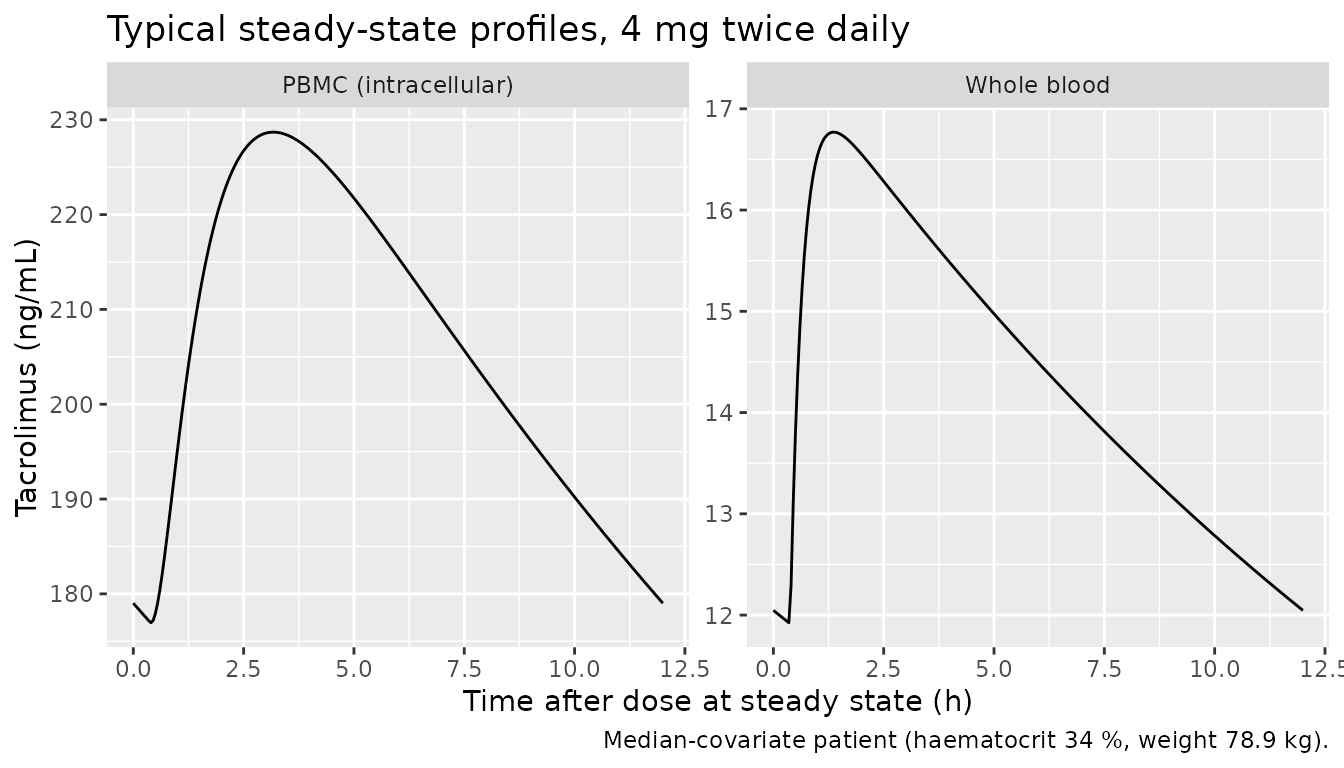
The PBMC concentration is about 14 times the whole-blood concentration and lags it. With = 0.9 1/h the equilibration half-life is 0.77 h, which is short against the 12 h dosing interval but long enough to blunt the absorption peak.
Replicate Figure 4 and Supplementary Table S1
The Supplementary Table S1 interquartile ranges are as wide as the
38.9 % inter-individual variability of ppc alone predicts.
For example, the IC IQR at haematocrit 0.28 is 0.77-1.28 times the
median, against exp(-/+0.674 x 0.375) = 0.78-1.29. So the published
simulation varied only that random effect and kept the whole-blood layer
at its typical values. The replication does the same: the whole-blood
etas are set to zero and 200 patients are simulated per scenario.
The paper calls these steady-state pre-dose concentrations but gives neither the dose nor the number of doses. Each published IC median times its ratio gives the whole-blood trough the paper simulated. Relative to the median scenario, those troughs match a dose train of about one week much better than the true periodic steady state (next table). The terminal phase of the Andrews 2019 model is slow, so the covariates that move CL/F (haematocrit, and BSA through body weight) keep pulling the troughs apart for weeks after the covariates that move V1/F have settled. The replication therefore uses 14 doses, 7 days of twice-daily dosing, and reads the trough just before dose 15. The true steady state is shown beside it.
ev_typ <- function(n_doses) {
  dplyr::bind_rows(lapply(seq_len(nrow(scenarios)), function(i) {
    make_events(scenarios[i, ], id_offset = i - 1L, n_doses = n_doses)
  }))
}
solve_trough <- function(n_doses, t_obs) {
  rxode2::rxSolve(
    mod, ev_typ(n_doses), omega = NA, sigma = NA, returnType = "data.frame",
    useLinCmt = FALSE, maxsteps = 500000L, keep = "scenario"
  ) |>
    dplyr::filter(time == t_obs) |>
    dplyr::transmute(scenario = as.character(scenario), Cc, Cpbmc,
                     r_typ = Cc / Cpbmc)
}
n_doses_fig4 <- 14L
typ_week <- solve_trough(n_doses_fig4, n_doses_fig4 * tau)
typ_ss <- solve_trough(NULL, tau)

published_s1 <- tibble::tribble(
  ~scenario, ~ic_med, ~ic_q1, ~ic_q3, ~r_med, ~r_q1, ~r_q3,
  "Haematocrit 0.28 L/L", 199.2, 154.1, 255.8, 0.054, 0.042, 0.069,
  "Haematocrit 0.34 L/L", 181.6, 140.6, 233.3, 0.068, 0.053, 0.087,
  "Haematocrit 0.43 L/L", 168.2, 124.1, 217.9, 0.081, 0.063, 0.110,
  "Weight 58.5 kg",       160.1, 123.8, 205.5, 0.080, 0.062, 0.104,
  "Weight 78.9 kg",       186.1, 144.0, 239.1, 0.066, 0.051, 0.085,
  "Weight 102 kg",        201.2, 148.4, 260.5, 0.057, 0.044, 0.078
) |>
  dplyr::mutate(
    wb_med = ic_med * r_med,
    ref = ifelse(grepl("^Haem", scenario), "Haematocrit 0.34 L/L", "Weight 78.9 kg")
  )

relative_to_ref <- function(d, col) {
  d |>
    dplyr::select(-dplyr::any_of("ref")) |>
    dplyr::left_join(published_s1[, c("scenario", "ref")], by = "scenario") |>
    dplyr::group_by(ref) |>
    dplyr::mutate(rel = .data[[col]] / .data[[col]][scenario == ref]) |>
    dplyr::ungroup() |>
    dplyr::pull(rel)
}
wb_rel <- tibble::tibble(
  scenario = published_s1$scenario,
  published = relative_to_ref(published_s1, "wb_med"),
  week = relative_to_ref(typ_week, "Cc"),
  steady = relative_to_ref(typ_ss, "Cc")
)
wb_rel |>
  dplyr::mutate(dplyr::across(-scenario, ~ sprintf("%.3f", .x))) |>
  dplyr::rename(
    "Scenario" = scenario,
    "Published (IC x WB:IC)" = published,
    "Simulated, 7 days" = week,
    "Simulated, true steady state" = steady
  ) |>
knitr::kable(caption = "Whole-blood trough relative to each panel's median scenario.")| Scenario | Published (IC x WB:IC) | Simulated, 7 days | Simulated, true steady state |
|---|---|---|---|
| Haematocrit 0.28 L/L | 0.871 | 0.873 | 0.839 |
| Haematocrit 0.34 L/L | 1.000 | 1.000 | 1.000 |
| Haematocrit 0.43 L/L | 1.103 | 1.163 | 1.231 |
| Weight 58.5 kg | 1.043 | 1.044 | 1.108 |
| Weight 78.9 kg | 1.000 | 1.000 | 1.000 |
| Weight 102 kg | 0.934 | 0.940 | 0.903 |
ok <- published_s1$scenario != "Haematocrit 0.43 L/L"
stopifnot(
  # The one-week train tracks the published troughs to under 1 %; the true
  # steady state misses the outer scenarios by 3-6 %. Both are deterministic.
  max(abs(wb_rel$week[ok] / wb_rel$published[ok] - 1)) < 0.03,
  max(abs(wb_rel$steady[ok] / wb_rel$published[ok] - 1)) >
    max(abs(wb_rel$week[ok] / wb_rel$published[ok] - 1))
)
mod_ppc_only <- mod |>
  rxode2::ini(etalcl = 0, etalvc = 0, etalvp = 0, etalq = 0)
#> ℹ parameter labels from comments will be replaced by 'label()'
#> ℹ change initial estimate of `etalcl` to `0`
#> ℹ change initial estimate of `etalvc` to `0`
#> ℹ change initial estimate of `etalvp` to `0`
#> ℹ change initial estimate of `etalq` to `0`

n_per <- 200L
ev_fig4 <- dplyr::bind_rows(lapply(seq_len(nrow(scenarios)), function(i) {
  make_events(scenarios[i, ], n = n_per, id_offset = (i - 1L) * n_per,
              n_doses = n_doses_fig4)
}))
stopifnot(!anyDuplicated(unique(ev_fig4[, c("id", "time", "evid")])))

rxode2::rxSetSeed(20220420)
sim_fig4 <- rxode2::rxSolve(
  mod_ppc_only, ev_fig4, sigma = NA, returnType = "data.frame",
  useLinCmt = FALSE, maxsteps = 500000L, keep = c("scenario", "panel")
)
#> ℹ omega/sigma items treated as zero: 'etalcl', 'etalvc', 'etalvp', 'etalq'
trough <- sim_fig4 |>
  dplyr::filter(time == n_doses_fig4 * tau) |>
  dplyr::mutate(ratio = Cc / Cpbmc)
stopifnot(nrow(trough) == n_per * nrow(scenarios), !anyNA(trough$ratio))
ggplot(trough, aes(scenario, ratio)) +
  geom_boxplot(outlier.size = 0.6) +
  facet_wrap(~panel, scales = "free_x") +
  labs(x = NULL, y = "Tacrolimus WB:IC ratio",
       title = "Whole-blood to intracellular ratio at the pre-dose trough",
       caption = "Replicates Figure 4 of Franken 2022 (200 simulated patients per scenario, day 7).") +
  theme(axis.text.x = element_text(angle = 20, hjust = 1))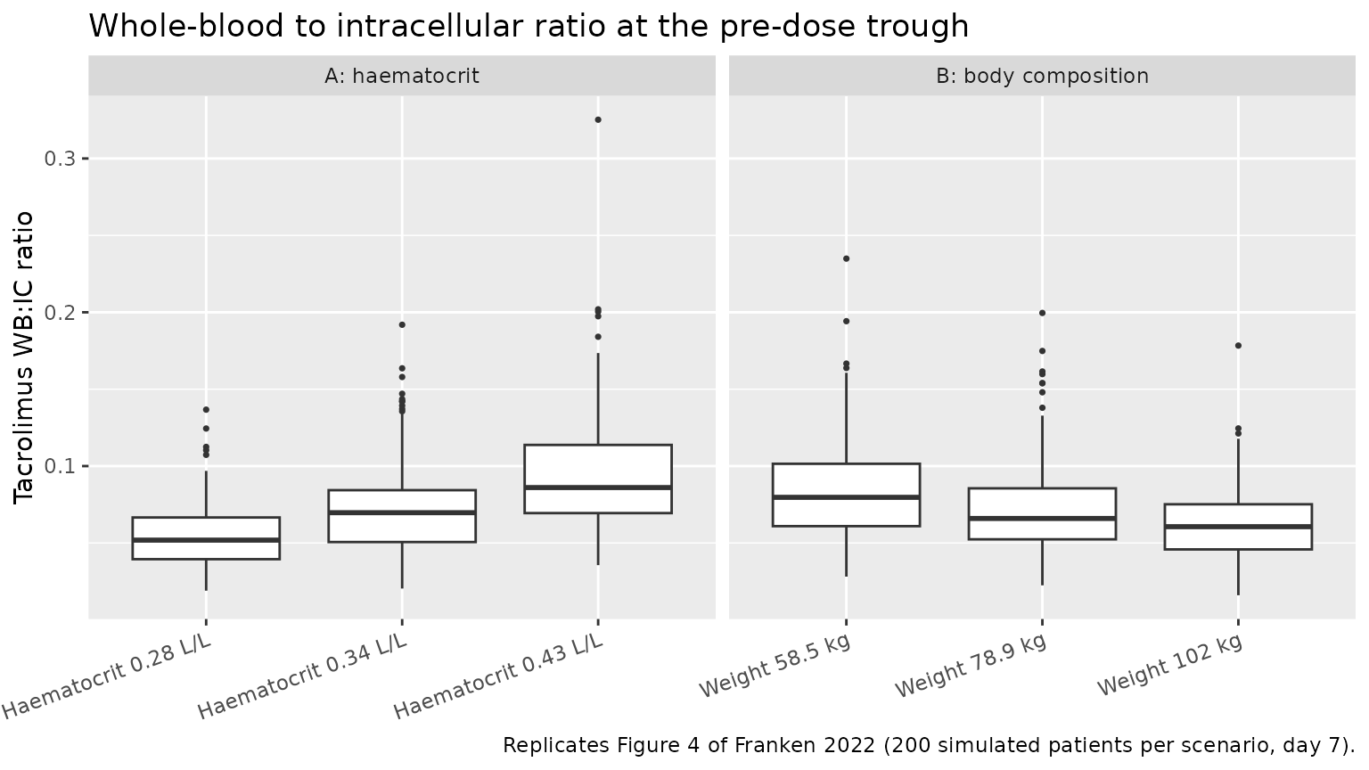
Supplementary Table S1 reports the ratio as whole blood over
intracellular, the reciprocal of ppc. The typical-value
ratio is exact, because it comes from a solve with no random effects.
The stochastic median and IQR come from the 200-patient simulation. The
ratio barely depends on how long dosing has run: it is ppc
scaled by a small lag factor from the effect compartment.
s1 <- trough |>
  dplyr::group_by(scenario = as.character(scenario)) |>
  dplyr::summarise(
    r_sim = median(ratio),
    r_sim_q1 = quantile(ratio, 0.25), r_sim_q3 = quantile(ratio, 0.75),
    .groups = "drop"
  ) |>
  dplyr::left_join(typ_week |> dplyr::select(scenario, r_typ, ic_typ = Cpbmc),
                   by = "scenario") |>
  dplyr::left_join(typ_ss |> dplyr::select(scenario, r_ss = r_typ),
                   by = "scenario") |>
  dplyr::left_join(published_s1, by = "scenario") |>
  dplyr::mutate(
    scenario = factor(scenario, levels = levels(scenarios$scenario)),
    pct_diff = 100 * (r_typ / r_med - 1)
  ) |>
  dplyr::arrange(scenario)

s1 |>
  dplyr::transmute(
    Scenario = scenario,
    `Published WB:IC, median (IQR)` = sprintf("%.3f (%.3f-%.3f)", r_med, r_q1, r_q3),
    `Simulated WB:IC, median (IQR)` = sprintf("%.3f (%.3f-%.3f)", r_sim, r_sim_q1, r_sim_q3),
    `Typical WB:IC, 7 days` = sprintf("%.4f", r_typ),
    `Typical WB:IC, steady state` = sprintf("%.4f", r_ss),
    `Typical (7 days) vs published (%)` = sprintf("%+.1f", pct_diff)
  ) |>
knitr::kable(caption = "Whole-blood:intracellular ratio at the pre-dose trough versus Supplementary Table S1.")| Scenario | Published WB:IC, median (IQR) | Simulated WB:IC, median (IQR) | Typical WB:IC, 7 days | Typical WB:IC, steady state | Typical (7 days) vs published (%) |
|---|---|---|---|---|---|
| Haematocrit 0.28 L/L | 0.054 (0.042-0.069) | 0.052 (0.039-0.067) | 0.0520 | 0.0528 | -3.7 |
| Haematocrit 0.34 L/L | 0.068 (0.053-0.087) | 0.070 (0.051-0.084) | 0.0663 | 0.0673 | -2.5 |
| Haematocrit 0.43 L/L | 0.081 (0.063-0.110) | 0.086 (0.069-0.114) | 0.0888 | 0.0901 | +9.6 |
| Weight 58.5 kg | 0.080 (0.062-0.104) | 0.080 (0.061-0.101) | 0.0797 | 0.0814 | -0.3 |
| Weight 78.9 kg | 0.066 (0.051-0.085) | 0.066 (0.052-0.086) | 0.0663 | 0.0673 | +0.4 |
| Weight 102 kg | 0.057 (0.044-0.078) | 0.061 (0.046-0.075) | 0.0589 | 0.0596 | +3.3 |
Five of the six scenarios reproduce the published median ratio to
within a few percent. The exception is the 90th-percentile haematocrit,
0.43 L/L, where the model gives a ratio about 10 % above the published
0.081. Equation 4 fixes that value at (43 / 34)^1.22 times
the reference ratio, so neither the dose nor the dosing duration can
bring it down to 0.081. Both the published ratio and the published
whole-blood trough for that row fit a haematocrit of about 0.40 L/L
instead (see Assumptions and deviations).
ok <- s1$scenario != "Haematocrit 0.43 L/L"
stopifnot(
  # Typical-value ratio: deterministic, so a tight bound. A mis-transcribed
  # ppc, exponent or centring value moves these by tens of percent.
  max(abs(s1$pct_diff[ok])) < 6,
  # Stochastic median: 200 patients give a Monte-Carlo SE of about 3 %.
  max(abs(s1$r_sim[ok] / s1$r_med[ok] - 1)) < 0.12,
  # IQR width tests the eta variance: the published q3/q1 ratios are
  # 1.64-1.77, and the simulated ones carry about 5 % Monte-Carlo noise.
  abs(log(median(s1$r_sim_q3 / s1$r_sim_q1) / median(s1$r_q3 / s1$r_q1))) < 0.2
)
The absolute IC concentration depends on the dose, which is not reported. The table compares IC concentrations relative to each panel’s median scenario.
ic_rel <- tibble::tibble(
  scenario = published_s1$scenario,
  published = relative_to_ref(published_s1, "ic_med"),
  simulated = relative_to_ref(typ_week, "Cpbmc")
)
ic_rel |>
  dplyr::transmute(
    Scenario = scenario,
    `Published IC relative to median scenario` = sprintf("%.3f", published),
    `Simulated IC relative to median scenario (7 days)` = sprintf("%.3f", simulated)
  ) |>
knitr::kable(caption = "Intracellular trough concentration relative to the median-covariate scenario of each panel.")| Scenario | Published IC relative to median scenario | Simulated IC relative to median scenario (7 days) |
|---|---|---|
| Haematocrit 0.28 L/L | 1.097 | 1.113 |
| Haematocrit 0.34 L/L | 1.000 | 1.000 |
| Haematocrit 0.43 L/L | 0.926 | 0.869 |
| Weight 58.5 kg | 0.860 | 0.868 |
| Weight 78.9 kg | 1.000 | 1.000 |
| Weight 102 kg | 1.081 | 1.058 |
ok_ic <- ic_rel$scenario != "Haematocrit 0.43 L/L"
# The published IC medians are Monte-Carlo medians of 1000 patients (about
# 2.5 % SE each), so a ratio of two of them carries about 3.5 % noise.
stopifnot(max(abs(ic_rel$simulated[ok_ic] / ic_rel$published[ok_ic] - 1)) < 0.08)
With 4 mg twice daily for 7 days, the median-covariate patient has a typical whole-blood trough of 8.1 ng/mL. The published values imply about 12.3 ng/mL, so the paper’s unstated dose was higher than the one used here. Absolute concentrations scale with the dose; none of the comparisons above depends on it.
PKNCA validation
The paper reports no NCA. The interval below runs over one steady-state dosing interval for each typical-value scenario, separately for each matrix. At steady state the effect compartment returns to its starting value over the interval. Integrating Equation 3 over the interval then gives exactly, which checks the effect-compartment wiring independently of the published numbers.
ev_nca <- dplyr::bind_rows(lapply(seq_len(nrow(scenarios)), function(i) {
  make_events(scenarios[i, ], id_offset = i - 1L, grid = grid)
}))
sim_nca <- rxode2::rxSolve(
  mod, ev_nca, omega = NA, sigma = NA, returnType = "data.frame",
  useLinCmt = FALSE, maxsteps = 500000L, keep = "scenario"
) |>
  dplyr::mutate(scenario = as.character(scenario))

dose_df <- ev_nca |>
  dplyr::filter(evid == 1) |>
  dplyr::transmute(id, time, amt, scenario = as.character(scenario))
intervals <- data.frame(start = 0, end = tau, cmax = TRUE, tmax = TRUE,
                        cmin = TRUE, auclast = TRUE)

run_nca <- function(conc_col) {
  conc <- sim_nca |>
    dplyr::filter(!is.na(.data[[conc_col]])) |>
    dplyr::transmute(id, time, scenario, conc = .data[[conc_col]])
  dat <- PKNCA::PKNCAdata(
    PKNCA::PKNCAconc(conc, conc ~ time | scenario + id),
    PKNCA::PKNCAdose(dose_df, amt ~ time | scenario + id),
    intervals = intervals
  )
  as.data.frame(PKNCA::pk.nca(dat)) |>
    dplyr::select(scenario, PPTESTCD, PPORRES) |>
    tidyr::pivot_wider(names_from = PPTESTCD, values_from = PPORRES)
}
nca_wb <- run_nca("Cc")
nca_ic <- run_nca("Cpbmc")

ppc_typ <- sim_nca |> dplyr::distinct(scenario, ppc)
nca_tab <- nca_wb |>
  dplyr::inner_join(nca_ic, by = "scenario", suffix = c("_wb", "_ic")) |>
  dplyr::inner_join(ppc_typ, by = "scenario") |>
  dplyr::mutate(
    scenario = factor(scenario, levels = levels(scenarios$scenario)),
    auc_ratio = auclast_ic / auclast_wb
  ) |>
  dplyr::arrange(scenario)

nca_tab |>
  dplyr::select(scenario, cmax_wb, cmin_wb, auclast_wb, cmax_ic, cmin_ic,
                auclast_ic, auc_ratio, ppc) |>
  dplyr::rename(
    "Scenario" = scenario,
    "WB Cmax (ng/mL)" = cmax_wb, "WB Cmin (ng/mL)" = cmin_wb,
    "WB AUCtau (ng*h/mL)" = auclast_wb,
    "IC Cmax (ng/mL)" = cmax_ic, "IC Cmin (ng/mL)" = cmin_ic,
    "IC AUCtau (ng*h/mL)" = auclast_ic,
    "AUC IC/WB" = auc_ratio, "ppc" = ppc
  ) |>
knitr::kable(digits = 3, caption = "Steady-state NCA (PKNCA) over one 12 h interval, 4 mg twice daily, typical values.")| Scenario | WB Cmax (ng/mL) | WB Cmin (ng/mL) | WB AUCtau (ng*h/mL) | IC Cmax (ng/mL) | IC Cmin (ng/mL) | IC AUCtau (ng*h/mL) | AUC IC/WB | ppc |
|---|---|---|---|---|---|---|---|---|
| Haematocrit 0.28 L/L | 14.822 | 9.984 | 148.273 | 254.169 | 188.738 | 2699.857 | 18.209 | 18.209 |
| Haematocrit 0.34 L/L | 16.769 | 11.924 | 171.848 | 228.696 | 176.953 | 2469.175 | 14.368 | 14.369 |
| Haematocrit 0.43 L/L | 19.550 | 14.697 | 205.425 | 201.841 | 162.902 | 2216.334 | 10.789 | 10.789 |
| Weight 58.5 kg | 19.669 | 13.191 | 196.024 | 218.604 | 161.778 | 2316.900 | 11.819 | 11.820 |
| Weight 78.9 kg | 16.769 | 11.924 | 171.848 | 228.696 | 176.953 | 2469.175 | 14.368 | 14.369 |
| Weight 102 kg | 14.812 | 10.779 | 153.488 | 229.282 | 180.549 | 2493.773 | 16.247 | 16.247 |
Simulated cohort versus the reported individual ratios
Section 3.6 gives the median individual
as 14371 (IQR 13060-17937) in the 16 patients with biopsy-proven acute
rejection and 12274 (IQR 10708-15159) in the 158 without. These are
empirical Bayes estimates on the paper’s scale, which is
ppc x 1000. Below they are set beside the ppc
distribution of a virtual cohort whose lean body mass and haematocrit
are drawn to match the Table 1 medians and IQRs. Empirical Bayes
estimates are pulled towards the typical value (33 % shrinkage, Table
2), so this is a context check rather than a gate.
set.seed(2022)
n_cohort <- 200L
# Log-normal draws whose median and IQR match Table 1: LBW 60.9 (53.8-66.9) kg,
# haematocrit 0.34 (0.31-0.38) L/L. The IQR/1.349 rule converts the log-scale
# IQR to a standard deviation.
cohort <- tibble(
  id = seq_len(n_cohort),
  LBM = exp(rnorm(n_cohort, log(60.9), log(66.9 / 53.8) / 1.349)),
  HCT = 100 * exp(rnorm(n_cohort, log(0.34), log(0.38 / 0.31) / 1.349))
)
eta_ppc <- rnorm(n_cohort, 0, sqrt(0.140910))
cohort$ppc_x1000 <- 1000 * (14100 / 1000) * exp(eta_ppc) *
  (cohort$LBM / 59.5)^1.01 * (cohort$HCT / 34)^-1.22

tibble::tibble(
  Source = c("Simulated cohort (n = 200)", "Reported, no BPAR (n = 158)",
             "Reported, BPAR (n = 16)"),
  `Median R WB:IC` = c(median(cohort$ppc_x1000), 12274, 14371),
  `Q1` = c(quantile(cohort$ppc_x1000, 0.25), 10708, 13060),
  `Q3` = c(quantile(cohort$ppc_x1000, 0.75), 15159, 17937)
) |>
knitr::kable(digits = 0, caption = "Individual R WB:IC (ppc x 1000) in a virtual cohort and as reported in Section 3.6.")| Source | Median R WB:IC | Q1 | Q3 |
|---|---|---|---|
| Simulated cohort (n = 200) | 14285 | 10907 | 19632 |
| Reported, no BPAR (n = 158) | 12274 | 10708 | 15159 |
| Reported, BPAR (n = 16) | 14371 | 13060 | 17937 |
The simulated median sits close to the typical value of 14100, as it must. The reported median of the 158 patients without rejection is about 14 % lower, and both reported IQRs are narrower than the simulated one. Narrower spread is what 33 % shrinkage does to empirical Bayes estimates, so the comparison does not test the model. It does show that the population typical value lies inside the range of the individual estimates the paper reports.
Assumptions and deviations
-
Whole-blood layer. Franken 2022 fixed the
whole-blood parameters at each patient’s individual Andrews 2019
estimates. A library model has no individual estimates, so the
whole-blood layer here is the Andrews 2019 population model: its typical
values, covariate effects and IIV, as printed in Franken 2022 Table 2.
The CL/F and V1/F centring values do not appear in Franken 2022. They
are the Andrews 2019 Supporting Information control-stream constants and
are carried from
Andrews_2019_tacrolimus. -
Whole-blood residual error. Franken 2022
re-estimated a proportional-only whole-blood error of 61.1 % (Data S1
CMT.EQ.2branch). It is much larger than the Andrews 2019 immunoassay error (17.7 % plus 0.88 ng/mL) because the individual whole-blood parameters carried no inter-occasion terms. That value is kept here as the paper’s estimate. For whole-blood-only simulation,Andrews_2019_tacrolimuscarries the better whole-blood error model. -
Inter-occasion variability. Table 2 lists the
Andrews 2019 IOV on CL/F (13.6 %), but Franken 2022 did not estimate it
and its control stream has no IOV term. It is not encoded, as in
Andrews_2019_tacrolimus. A user who needs it can add a per-occasion eta on CL/F with variance log(1 + 0.136^2) = 0.0184. -
Units of R WB:IC. In the control stream
RPICmultiplies the whole-blood concentration in mg/L (A(2)/V2, dose in mg and volume in L). The intracellular state is in ug/L (Supplementary Table S1). The estimate 14100 therefore carries a factor of 1000. This model drives the effect compartment withCcin ng/mL (= ug/L), soppc= 14100 / 1000 = 14.1, the “14-fold higher concentration in the PBMCs” of Results 3.2. - Ratio naming in the paper. Table 2 and Equation 4 call the estimated quantity , but it is the intracellular:whole-blood ratio (14.1). Supplementary Table S1 and Figure 4 report its reciprocal, whole blood over intracellular (about 0.07). The abstract and Section 3.5 describe the effects in that reciprocal sense: the WB:IC ratio rises with haematocrit and falls with body weight. The Section 3.3 sentence “LBW was positively correlated and haematocrit negatively correlated with the WB:IC ratio” matches the sign of the estimated exponents in Equation 4 (+1.01 and -1.22) instead. The maintainers coded Equation 4 and the control stream, which agree with each other and with Supplementary Table S1.
-
Haematocrit scale. The paper records haematocrit in
L/L. The canonical
HCTcolumn is in percent, so both centring values (0.34 L/L) are 34 here. -
Rounded constants. The control stream hardcodes
KA = 3.6andALAG1 = 0.382. Table 2 prints 3.58 and 0.38, which are also the Andrews 2019 values, and this model uses those. The difference is below 1 %. - Simulated patient. Figure 4B prints weight, LBW and BSA for each body-composition scenario. Those values identify a male patient 174.5 cm tall, and that patient is used for all six scenarios. Age, albumin and creatinine are the Table 1 medians. CYP3A5 and CYP3A4 genotypes are the reference categories. The simulated dose (4 mg twice daily) is an assumption, since the paper does not state it.
- Dosing duration for Figure 4. The paper calls the Figure 4 and Supplementary Table S1 troughs “steady state” without stating how long it dosed. The relative whole-blood troughs implied by Supplementary Table S1 match 5-10 days of twice-daily dosing to about 1 %. At the true periodic steady state the outer scenarios miss by 3-6 %. The maintainers therefore replicate the figure at day 7 (14 doses) and show the true steady state alongside. The WB:IC ratio itself changes by about 2 % between the two.
- Haematocrit 0.43 L/L scenario. The published ratio for the 90th-percentile haematocrit (0.081) is about 10 % below what Equation 4 gives at 0.43 L/L. Its published whole-blood trough (IC median x ratio, 13.6 ng/mL) also falls short of the haematocrit effect on CL/F. Both published quantities fit a haematocrit near 0.40 L/L. This is recorded as a deviation of the published table and excluded from the gate. The model was not adjusted.
- Table 1 typo. Glucocorticoid co-medication is printed as “185 (100%)” in a cohort of 184.
- Literature check. No correction or erratum for Franken 2022 was found in Europe PMC or Crossref as of 2026-10-02.