Turoctocog alfa pegol subcutaneous PK in mouse, monkey and human (Rode 2018)
Source:vignettes/articles/Rode_2018_turoctocogAlfaPegol.Rmd
Rode_2018_turoctocogAlfaPegol.RmdModel and source
Rode et al. (2018) studied subcutaneous (SC) administration of turoctocog alfa pegol (N8-GP), a glycoPEGylated extended-half-life recombinant factor VIII. The paper fits two preclinical population PK models – FVIII knockout mice and cynomolgus monkeys, each fitted to simultaneous SC and intravenous (IV) data – and then builds a human prediction model by combining the monkey SC absorption parameters with human clearance and volume from the IV pathfinder 1 trial. The three models are independent fits, so each is a separate model file:
Rode_2018_turoctocogAlfaPegol_mouse– one compartment, Table S1.Rode_2018_turoctocogAlfaPegol_cyno– two compartments with dose and formulation covariates, Table S2.Rode_2018_turoctocogAlfaPegol_human– one compartment, Table S3 plus the Table S2 absorption parameters.Citation: Rode F, Almholt K, Petersen M, Kreilgaard M, Kjalke M, Karpf DM, Groth AV, Johansen PB, Larsen LF, Loftager M, Haaning J. Preclinical pharmacokinetics and biodistribution of subcutaneously administered glycoPEGylated recombinant factor VIII (N8-GP) and development of a human pharmacokinetic prediction model. J Thromb Haemost. 2018;16(6):1141-1152. doi:10.1111/jth.14013. Clearance, volume and residual error from Table S3 (pathfinder 1, NCT01205724; Tiede A et al. J Thromb Haemost 2013;11:670-678, doi:10.1111/jth.12161, and data on file); ka and F from Table S2.
Article: https://doi.org/10.1111/jth.14013
Supplement (Data S1, Tables S1-S3): published with the article as
jth14013-sup-0001-Supinfo.docx.
All three models are parameterised per kg of body weight, so doses are in IU/kg and FVIII activity (FVIII:C) is in IU/mL; 1 IU/mL is 100% of normal.
Population
- Mice: FVIII exon 16 knockout (B6.129S4-F8tm1Kaz/J), male and female, 12-16 weeks. Three groups of 9 mice received 2500 IU/kg SC (flank, neck or lower abdomen) and 9 mice received 280 IU/kg IV; sparse sampling from 1 to 72 h (Methods, “PK studies in F8-KO mice”; Data S1).
- Cynomolgus monkeys: six monkeys received 100 IU/kg SC once daily on days 1-3 as either a 500 IU/mL (0.2 mL/kg, n = 3) or a 5000 IU/mL (0.02 mL/kg, n = 3) solution; five received a single IV dose of 100 IU/kg (n = 2) or 250 IU/kg (n = 3). Sampling over 96 h with an N8-GP-specific (anti-PEG capture) chromogenic assay.
- Humans: clearance and volume come from pathfinder 1 (NCT01205724), in which 26 patients with severe haemophilia A received single IV doses of 25, 50 or 75 IU/kg. Rode 2018 does not tabulate their demographics; Table S3 reports parameters “for a 70-kg individual”.
lapply(
  c("Rode_2018_turoctocogAlfaPegol_mouse", "Rode_2018_turoctocogAlfaPegol_cyno",
    "Rode_2018_turoctocogAlfaPegol_human"),
  function(nm) readModelDb(nm)()$population$species
)
#> [[1]]
#> [1] "mouse (FVIII exon 16 knockout, B6.129S4-F8tm1Kaz/J)"
#>
#> [[2]]
#> [1] "monkey (cynomolgus, Macaca fascicularis)"
#>
#> [[3]]
#> [1] "human"
Source trace
| Model | Parameter | Value | Source location |
|---|---|---|---|
| mouse |
lvc (V/Bw) |
log(39 mL/kg) | Table S1 |
| mouse |
lkel (Ke) |
log(0.049 1/h) | Table S1 |
| mouse |
lka (Ka) |
log(0.094 1/h) | Table S1 |
| mouse |
lfdepot (F) |
log(0.24) | Table S1 (24%) |
| mouse | etalvc |
0.047268 = log(1 + 0.22^2) | Table S1, IIV on V/Bw 22% |
| mouse | propSd |
0.32 | Table S1 |
| mouse | structure: 1 compartment, first-order SC absorption, IIV on V only | n/a | Methods, “PK modeling” |
| cyno |
lvc (V/Bw) |
log(61 mL/kg) | Table S2 |
| cyno |
lcl (Cl/Bw) |
log(3.0 mL/h/kg) | Table S2 |
| cyno |
lvp (V2/Bw) |
log(15 mL/kg) | Table S2 |
| cyno |
lq (Cl2/Bw) |
log(1.2 mL/h/kg) | Table S2 |
| cyno |
lka (ka) |
log(0.33 1/h) | Table S2 |
| cyno |
lfdepot (F) |
log(0.26) | Table S2 (26%) |
| cyno | e_form_turoctocogpegol_soln5000_fdepot |
-0.32 | Table S2, “Relative effect of low SC dose volume on F” |
| cyno | e_dose_high_vc |
-0.49 | Table S2, “Relative effect of high IV dose on V” |
| cyno | e_dose_high_cl |
-0.29 | Table S2, “Relative effect of high IV dose on Cl” |
| cyno | etalka |
0.14177 = log(1 + 0.39^2) | Table S2, IIV 39% |
| cyno | etalfdepot |
0.019414 = log(1 + 0.14^2) | Table S2, IIV 14% |
| cyno | propSd |
0.39 | Table S2 |
| cyno | structure: 2 compartments, first-order SC absorption, IV dose covariate on V and CL, SC dose-volume covariate on F | n/a | Methods, “PK modeling” |
| human |
lcl (Cl/Bw) |
log(1.7 mL/h/kg) | Table S3 |
| human |
lvc (V/Bw) |
log(45 mL/kg) | Table S3 |
| human |
lka, lfdepot, etalka,
etalfdepot
|
as cyno | Table S2; Methods, “Human PK prediction model” |
| human | etalcl |
0.14842 = log(1 + 0.40^2) | Table S3, IIV 40% |
| human | etalvc |
0.060625 = log(1 + 0.25^2) | Table S3, IIV 25% |
| human | CL-V covariance | 0.022780 | Table S3, “Cl-V covariance” 24%, read as a correlation of 0.24 |
| human | propSd |
0.117 | Table S3 |
| human | structure: 1 compartment with first-order SC absorption | n/a | Methods, “Human PK prediction model” |
Mouse model
mod_mouse <- readModelDb("Rode_2018_turoctocogAlfaPegol_mouse")
obs_mouse <- c(seq(0, 12, by = 1), seq(14, 72, by = 2))

make_single <- function(n, amt, cmt, treatment, id_offset, obs_times) {
  ids <- id_offset + seq_len(n)
  dose <- tibble(id = ids, time = 0, amt = amt, evid = 1L, cmt = cmt)
  obs <- tidyr::expand_grid(id = ids, time = obs_times) |>
    mutate(amt = 0, evid = 0L, cmt = "central")
  bind_rows(dose, obs) |>
    mutate(treatment = treatment) |>
    arrange(id, time, desc(evid))
}

events_mouse <- bind_rows(
  make_single(200, 2500, "depot", "SC 2500 IU/kg", 0L, obs_mouse),
  make_single(200, 280, "central", "IV 280 IU/kg", 200L, obs_mouse)
)
stopifnot(!anyDuplicated(unique(events_mouse[, c("id", "time", "evid")])))

rxode2::rxSetSeed(2018)
sim_mouse <- rxode2::rxSolve(mod_mouse, events = events_mouse,
                             keep = "treatment") |>
  as.data.frame()
#> ℹ parameter labels from comments will be replaced by 'label()'
vpc_summary <- function(sim, by = "treatment") {
  sim |>
    group_by(across(all_of(c(by, "time")))) |>
    summarise(
      Q025 = quantile(Cc, 0.025, na.rm = TRUE),
      Q50 = quantile(Cc, 0.5, na.rm = TRUE),
      Q975 = quantile(Cc, 0.975, na.rm = TRUE),
      .groups = "drop"
    )
}

vpc_summary(sim_mouse) |>
  ggplot(aes(time, Q50)) +
  geom_ribbon(aes(ymin = Q025, ymax = Q975), fill = "grey70") +
  geom_line() +
  facet_wrap(~treatment, scales = "free_y") +
  scale_x_continuous(breaks = seq(0, 72, 24)) +
  labs(x = "Time (h)", y = "FVIII:C (IU/mL)")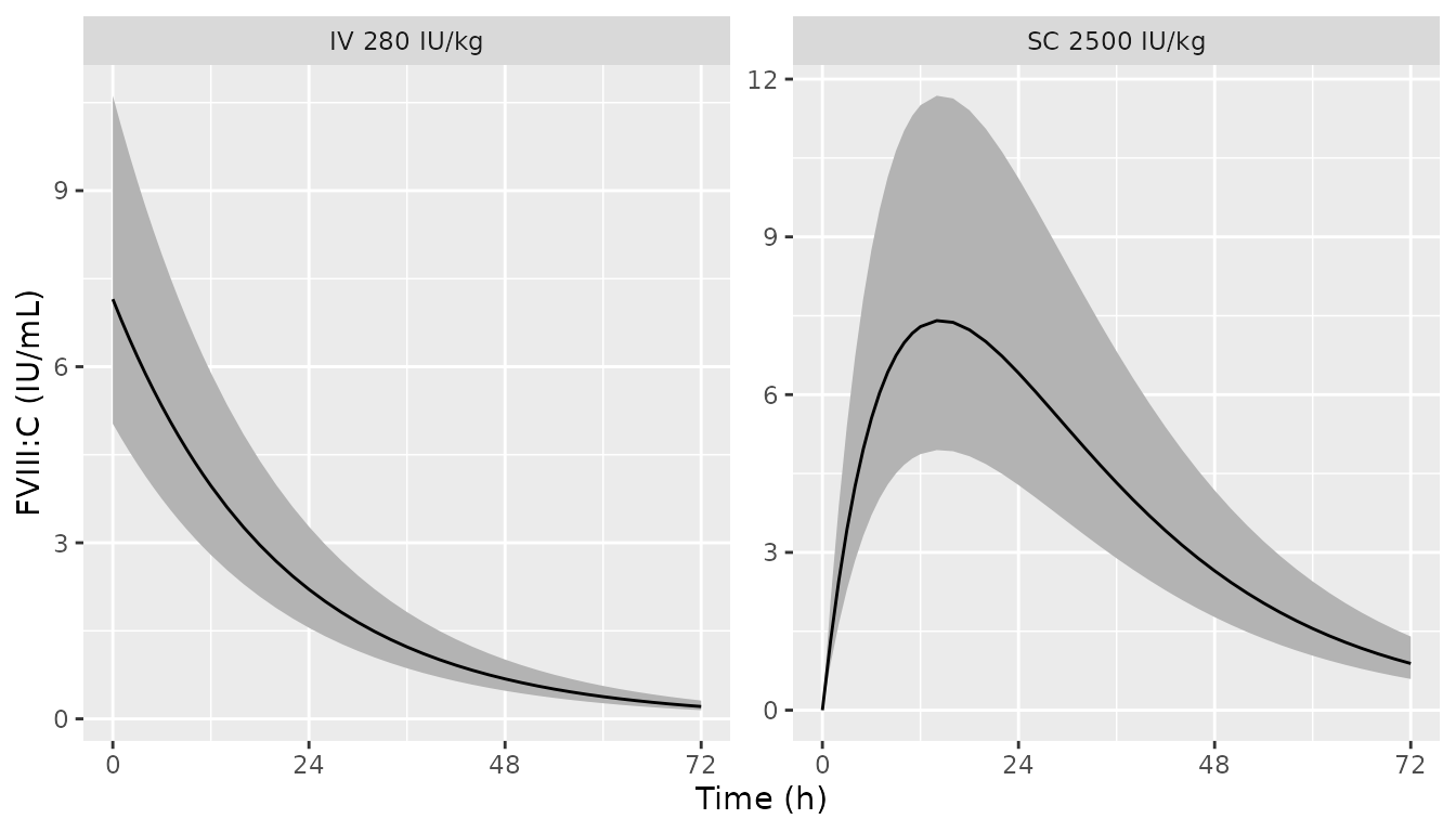
Replicates Figure 1 of Rode 2018: median and 95% prediction interval of FVIII:C after 2500 IU/kg SC (A) and 280 IU/kg IV (B) in F8-KO mice.
The published median SC profile peaks near 7 IU/mL around 18 h with the 95% band reaching about 12 IU/mL, and the IV median starts near 7 IU/mL; both are reproduced above.
The paper reports a SC Tmax of 14 h and a terminal half-life of 14 h. Both follow from the typical parameters in closed form, so they are checked exactly:
p_mouse <- with(as.list(rxode2::rxode(mod_mouse)$theta),
                c(ka = exp(lka), ke = exp(lkel)))
#> ℹ parameter labels from comments will be replaced by 'label()'
tmax_mouse <- log(p_mouse[["ka"]] / p_mouse[["ke"]]) /
  (p_mouse[["ka"]] - p_mouse[["ke"]])
thalf_mouse <- log(2) / p_mouse[["ke"]]
c(tmax_h = tmax_mouse, thalf_h = thalf_mouse)
#>   tmax_h  thalf_h
#> 14.47721 14.14586
stopifnot(
  abs(tmax_mouse - 14) < 1,
  abs(thalf_mouse - 14) < 0.5
)
Cynomolgus monkey model
mod_cyno <- readModelDb("Rode_2018_turoctocogAlfaPegol_cyno")
obs_cyno <- sort(unique(c(seq(0, 96, by = 1), 0.25, 0.5)))

make_cyno_sc <- function(n, form5000, treatment, id_offset) {
  ids <- id_offset + seq_len(n)
  dose <- tidyr::expand_grid(id = ids, time = c(0, 24, 48)) |>
    mutate(amt = 100, evid = 1L, cmt = "depot")
  obs <- tidyr::expand_grid(id = ids, time = obs_cyno) |>
    mutate(amt = 0, evid = 0L, cmt = "central")
  bind_rows(dose, obs) |>
    mutate(treatment = treatment, FORM_TUROCTOCOGPEGOL_SOLN5000 = form5000,
           DOSE_HIGH = 0L) |>
    arrange(id, time, desc(evid))
}
make_cyno_iv <- function(n, amt, treatment, id_offset) {
  # DOSE_HIGH = 1 only for the 250 IU/kg IV dose (Table S2)
  dose_high <- as.integer(amt == 250)
  make_single(n, amt, "central", treatment, id_offset, obs_cyno[obs_cyno <= 72]) |>
    mutate(FORM_TUROCTOCOGPEGOL_SOLN5000 = 0L, DOSE_HIGH = dose_high)
}

events_cyno <- bind_rows(
  make_cyno_sc(200, 0L, "SC 500 IU/mL", 0L),
  make_cyno_sc(200, 1L, "SC 5000 IU/mL", 200L),
  make_cyno_iv(200, 100, "IV 100 IU/kg", 400L),
  make_cyno_iv(200, 250, "IV 250 IU/kg", 600L)
)
stopifnot(!anyDuplicated(unique(events_cyno[, c("id", "time", "evid")])))
stopifnot(all(events_cyno$DOSE_HIGH[events_cyno$treatment == "IV 250 IU/kg"] == 1L))

rxode2::rxSetSeed(2018)
sim_cyno <- rxode2::rxSolve(mod_cyno, events = events_cyno,
                            keep = "treatment") |>
  as.data.frame()
#> ℹ parameter labels from comments will be replaced by 'label()'
sc_pooled <- sim_cyno |>
  filter(grepl("^SC", treatment)) |>
  mutate(panel = "A: SC 100 IU/kg x 3")
iv_pooled <- sim_cyno |>
  filter(grepl("^IV", treatment)) |>
  # 2 of 5 study animals at 100 IU/kg and 3 of 5 at 250 IU/kg
  filter((treatment == "IV 100 IU/kg" & id <= 400 + 80) |
           (treatment == "IV 250 IU/kg" & id <= 600 + 120)) |>
  mutate(Cc = ifelse(treatment == "IV 250 IU/kg", Cc * 100 / 250, Cc),
         panel = "B: IV, dose-normalised to 100 IU/kg")

bind_rows(sc_pooled, iv_pooled) |>
  vpc_summary(by = "panel") |>
  ggplot(aes(time, Q50)) +
  geom_ribbon(aes(ymin = Q025, ymax = Q975), fill = "grey70") +
  geom_line() +
  facet_wrap(~panel, scales = "free") +
  scale_x_continuous(breaks = seq(0, 96, 24)) +
  labs(x = "Time (h)", y = "FVIII:C (IU/mL)")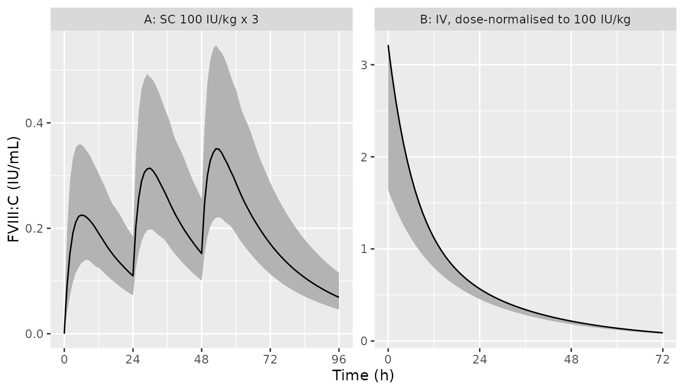
Replicates Figure 2 of Rode 2018: (A) 100 IU/kg SC on days 1-3, both formulations pooled 1:1 as in the study; (B) IV, dose-normalised to 100 IU/kg, both IV dose groups pooled as 2:3 (100:250 IU/kg) as in the study.
The published SC median rises to about 0.2, 0.3 and 0.35 IU/mL after the three doses, and the dose-normalised IV median starts near 2.8 IU/mL and falls below 0.5 IU/mL by 24 h. The pooled IV median is dominated by the 250 IU/kg animals, whose central volume is 49% smaller.
Formulation effect
The 5000 IU/mL (0.02 mL/kg) solution has 32% lower bioavailability than the 500 IU/mL (0.2 mL/kg) solution; the paper’s non-compartmental analysis found a 36% lower AUC. In a linear model the typical AUC ratio equals the F ratio:
cyno_typ <- rxode2::rxSolve(rxode2::zeroRe(mod_cyno),
                            events = events_cyno |> filter(id %in% c(1, 201)),
                            keep = "treatment") |>
  as.data.frame()
#> ℹ parameter labels from comments will be replaced by 'label()'
#> ℹ omega/sigma items treated as zero: 'etalka', 'etalfdepot'
#> Warning: multi-subject simulation without without 'omega'
auc_typ <- cyno_typ |>
  group_by(treatment) |>
  summarise(auc_0_96 = sum(diff(time) * (head(Cc, -1) + tail(Cc, -1)) / 2))
auc_typ
#> # A tibble: 2 × 2
#>   treatment     auc_0_96
#>   <chr>            <dbl>
#> 1 SC 500 IU/mL      23.5
#> 2 SC 5000 IU/mL     16.0
auc_ratio <- auc_typ$auc_0_96[auc_typ$treatment == "SC 5000 IU/mL"] /
  auc_typ$auc_0_96[auc_typ$treatment == "SC 500 IU/mL"]
stopifnot(abs(auc_ratio - 0.68) < 0.005)
NCA
PKNCA on the simulated cohorts: SC Tmax after the first dose (0-24 h) and IV terminal half-life (0-72 h).
conc_cyno <- sim_cyno |>
  filter(!is.na(Cc)) |>
  select(id, time, Cc, treatment)
conc_cyno <- bind_rows(
  conc_cyno,
  conc_cyno |> distinct(id, treatment) |> mutate(time = 0, Cc = 0)
) |>
  distinct(id, treatment, time, .keep_all = TRUE) |>
  arrange(treatment, id, time)
dose_cyno <- events_cyno |>
  filter(evid == 1) |>
  select(id, time, amt, treatment)

intervals_cyno <- bind_rows(
  data.frame(start = 0, end = 24, cmax = TRUE, tmax = TRUE, half.life = FALSE,
             treatment = c("SC 500 IU/mL", "SC 5000 IU/mL")),
  data.frame(start = 0, end = 72, cmax = TRUE, tmax = FALSE, half.life = TRUE,
             treatment = c("IV 100 IU/kg", "IV 250 IU/kg"))
)
nca_cyno <- PKNCA::pk.nca(PKNCA::PKNCAdata(
  PKNCA::PKNCAconc(conc_cyno, Cc ~ time | treatment + id),
  PKNCA::PKNCAdose(dose_cyno, amt ~ time | treatment + id),
  intervals = intervals_cyno
))

published_cyno <- tibble::tribble(
  ~treatment, ~tmax, ~half.life,
  "SC 500 IU/mL", 6.8, NA,
  "SC 5000 IU/mL", 6.8, NA,
  "IV 100 IU/kg", NA, 15,
  "IV 250 IU/kg", NA, 15
)
nlmixr2lib::ncaComparisonTable(
  simulated = nca_cyno,
  reference = published_cyno,
  by = "treatment",
  params = c("tmax", "half.life"),
  units = c(tmax = "h", half.life = "h"),
  tolerance_pct = 20
) |>
  # keep only the rows the paper reports
  dplyr::filter(grepl("^[0-9]", Reference)) |>
knitr::kable(caption = "Simulated (median) vs. published cynomolgus NCA. * differs from reference by >20%.")| NCA parameter | treatment | Reference | Simulated | % diff |
|---|---|---|---|---|
| Tmax (h) | SC 500 IU/mL | 6.8 | 6 | -11.8% |
| Tmax (h) | SC 5000 IU/mL | 6.8 | 6 | -11.8% |
| t½ (h) | IV 100 IU/kg | 15 | 19.6 | +30.9%* |
| t½ (h) | IV 250 IU/kg | 15 | 18.7 | +24.8%* |
The Tmax of 6.8 h is reproduced. The simulated half-life is starred:
the two-compartment model built from the Table S2 estimates has a
terminal half-life of about 20 h (log(2) over the slow
disposition rate constant, computed below), which PKNCA recovers from
the 0-72 h IV profiles, whereas the paper prints 15 h. The printed value
is closer to log(2) * V / CL, about 14 h, so it does not
appear to be the terminal phase of the fitted model. The parameters are
kept as published.
th_cyno <- rxode2::rxode(mod_cyno)$theta
#> ℹ parameter labels from comments will be replaced by 'label()'
k10 <- exp(th_cyno[["lcl"]]) / exp(th_cyno[["lvc"]])
k12 <- exp(th_cyno[["lq"]]) / exp(th_cyno[["lvc"]])
k21 <- exp(th_cyno[["lq"]]) / exp(th_cyno[["lvp"]])
beta <- ((k10 + k12 + k21) - sqrt((k10 + k12 + k21)^2 - 4 * k10 * k21)) / 2
c(terminal_thalf_h = log(2) / beta, ln2_V_over_CL_h = log(2) / k10)
#> terminal_thalf_h  ln2_V_over_CL_h
#>         20.16968         14.09399
Human prediction model
Figure 3 of the paper compares 12.5 IU/kg SC once daily with 50 IU/kg IV every fourth day over 9 days.
mod_human <- readModelDb("Rode_2018_turoctocogAlfaPegol_human")
obs_human <- sort(unique(c(seq(0, 216, by = 1), 191.99, 215.99)))

make_regimen <- function(n, amt, cmt, ii, ndose, treatment, id_offset) {
  ids <- id_offset + seq_len(n)
  dose <- tidyr::expand_grid(id = ids, time = ii * (seq_len(ndose) - 1)) |>
    mutate(amt = amt, evid = 1L, cmt = cmt)
  obs <- tidyr::expand_grid(id = ids, time = obs_human) |>
    mutate(amt = 0, evid = 0L, cmt = "central")
  bind_rows(dose, obs) |>
    mutate(treatment = treatment) |>
    arrange(id, time, desc(evid))
}

events_human <- bind_rows(
  make_regimen(200, 12.5, "depot", 24, 9, "SC 12.5 IU/kg q24h", 0L),
  make_regimen(200, 50, "central", 96, 3, "IV 50 IU/kg q4d", 200L)
)
stopifnot(!anyDuplicated(unique(events_human[, c("id", "time", "evid")])))

rxode2::rxSetSeed(2018)
sim_human <- rxode2::rxSolve(mod_human, events = events_human,
                             keep = "treatment") |>
  as.data.frame()
#> ℹ parameter labels from comments will be replaced by 'label()'
vpc_summary(sim_human) |>
  ggplot(aes(time / 24, Q50, linetype = treatment, fill = treatment)) +
  geom_ribbon(aes(ymin = Q025, ymax = Q975), alpha = 0.4) +
  geom_line() +
  scale_fill_manual(values = c("SC 12.5 IU/kg q24h" = "grey30",
                               "IV 50 IU/kg q4d" = "grey75")) +
  scale_linetype_manual(values = c("SC 12.5 IU/kg q24h" = "dashed",
                                   "IV 50 IU/kg q4d" = "solid")) +
  coord_cartesian(ylim = c(0, 0.2)) +
  scale_x_continuous(breaks = 0:9) +
  labs(x = "Time (day)", y = "FVIII:C (IU/mL)", fill = NULL, linetype = NULL)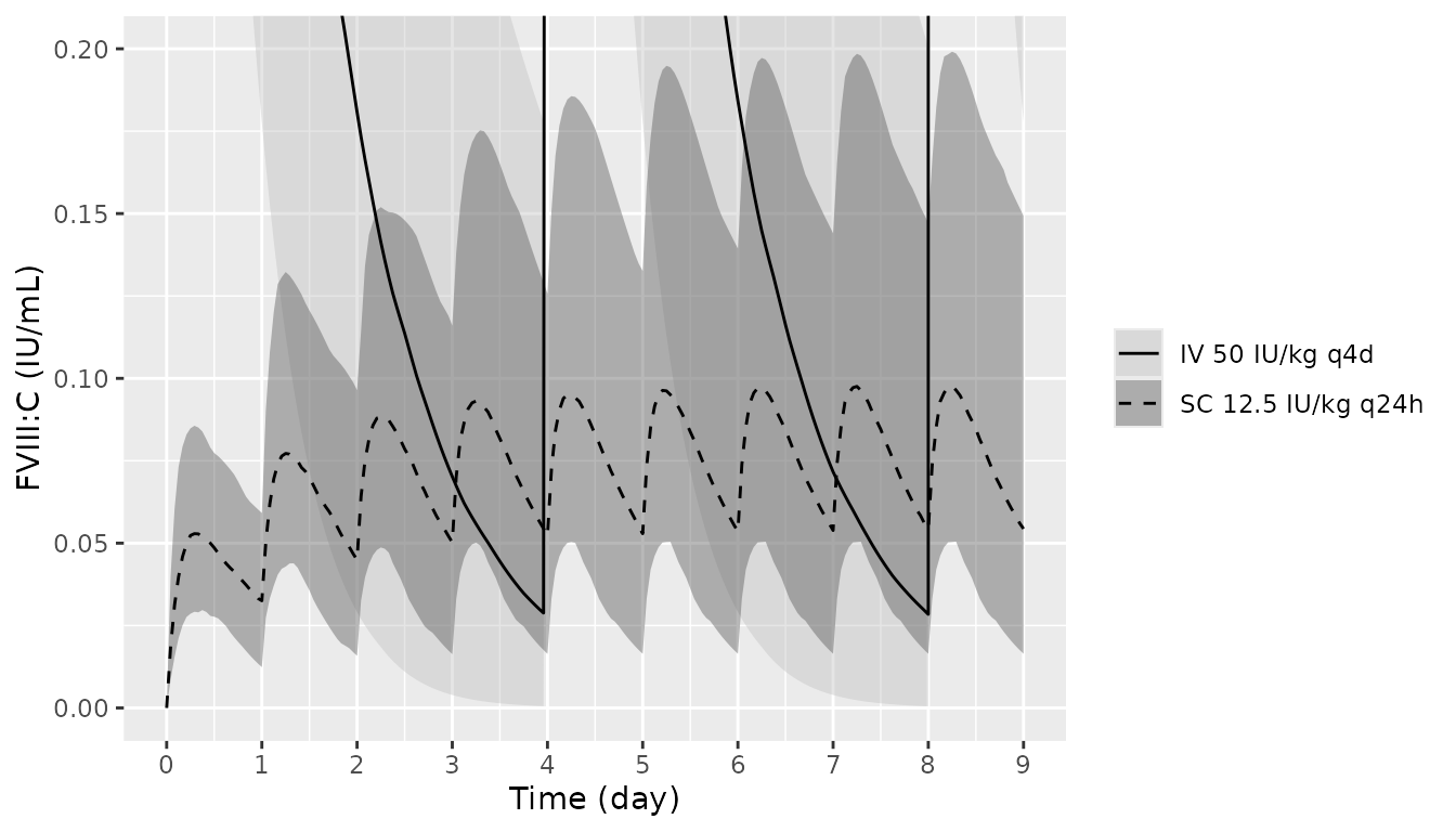
Replicates Figure 3 of Rode 2018: median and 95% prediction interval of FVIII:C for 12.5 IU/kg SC once daily (dashed, dark band) and 50 IU/kg IV every 4 days (solid, light band).
The typical steady-state average for the SC regimen is fixed by
F * dose / (CL * tau), which the typical-value solve must
reproduce:
th <- rxode2::rxode(mod_human)$theta
#> ℹ parameter labels from comments will be replaced by 'label()'
cavg_closed <- exp(th[["lfdepot"]]) * 12.5 / (exp(th[["lcl"]]) * 24)
typ_human <- rxode2::rxSolve(
  rxode2::zeroRe(mod_human), events = events_human |> filter(id == 1),
  keep = "treatment"
) |>
  as.data.frame() |>
  filter(time >= 192, time <= 216)
#> ℹ parameter labels from comments will be replaced by 'label()'
#> ℹ omega/sigma items treated as zero: 'etalcl', 'etalvc', 'etalka', 'etalfdepot'
cavg_sim <- sum(diff(typ_human$time) *
                  (head(typ_human$Cc, -1) + tail(typ_human$Cc, -1)) / 2) / 24
c(closed_form = cavg_closed, simulated_day9 = cavg_sim)
#>    closed_form simulated_day9
#>     0.07965686     0.07954853
stopifnot(abs(cavg_sim / cavg_closed - 1) < 0.02)
Day-9 trough and peak distributions for the SC regimen, against the paper’s statement that 12.5 IU/kg daily gives troughs of 2.5-10% and peaks of 5-15% in 95% of patients:
sc_day9 <- sim_human |>
  filter(treatment == "SC 12.5 IU/kg q24h", time > 192, time <= 216) |>
  group_by(id) |>
  summarise(trough = Cc[which.min(abs(time - 215.99))], peak = max(Cc))
tp <- rbind(
  trough = quantile(sc_day9$trough, c(0.025, 0.5, 0.975)),
  peak = quantile(sc_day9$peak, c(0.025, 0.5, 0.975))
)
knitr::kable(100 * tp, digits = 1,
caption = "Simulated day-9 SC FVIII:C (% of normal), 2.5th / 50th / 97.5th percentiles.")| 2.5% | 50% | 97.5% | |
|---|---|---|---|
| trough | 1.6 | 5.4 | 14.9 |
| peak | 5.1 | 9.8 | 19.9 |
iv_trough <- sim_human |>
  filter(treatment == "IV 50 IU/kg q4d", time == 191.99) |>
  pull(Cc)
quantile(iv_trough, c(0.025, 0.5, 0.975))
#>        2.5%         50%       97.5%
#> 0.000499442 0.028406139 0.200548321

stopifnot(
  # Medians read from Figure 3 at days 8-9: SC trough about 5.5%, IV trough
  # about 3.5%. The bounds allow for digitising error and cohort noise.
  median(sc_day9$trough) > 0.04, median(sc_day9$trough) < 0.07,
  median(iv_trough) > 0.02, median(iv_trough) < 0.05
)
The simulated medians match Figure 3. The simulated 95% range of SC troughs is wider than the 2.5-10% the paper states (see Assumptions and deviations).
Assumptions and deviations
-
IIV percentages. Tables S1-S3 give IIV as
percentages. They are read as coefficients of variation of log-normal
random effects, with
omega^2 = log(1 + CV^2). - Human CL-V covariance. Table S3 lists “Cl-V covariance 24%” in the IIV column. The maintainers read it as a correlation coefficient of 0.24 (covariance 0.0228). Reading it instead as a square-root-scale covariance (0.24^2 = 0.0576, a correlation of about 0.6) changes the 2.5th-97.5th percentiles of the simulated SC trough by less than 0.4 percentage points, so the choice is immaterial to every prediction shown here.
- Width of the human prediction interval. With the published IIV on CL (40%), V (25%), ka (39%) and F (14%), the simulated 95% range of steady-state SC troughs is roughly 1.5-15%, against the 2.5-10% stated in the abstract and Results; the paper’s Figure 3 band is also narrower than the simulated one. IIV on CL alone already produces a wider range than 2.5-10%, so no reading of the IIV percentages consistent with Table S3 reproduces the published width. The medians agree, and the parameters are kept as published.
- Human absorption parameters. Following the paper, ka, F and their IIV are the cynomolgus values for the reference 500 IU/mL formulation. The formulation covariate is not carried into the human model.
- Bioavailability random effect. The scale of the IIV on F is not stated; a log-normal random effect is used. With 14% CV the individual F stays far below 1.
-
Covariate effect form. “Relative effect” rows of
Table S2 are encoded as multiplicative factors
(1 + effect * indicator), so the typical values for the indicator = 1 groups are 0.68 x F, 0.51 x V and 0.71 x CL. - Mouse injection sites. The flank, neck and lower-abdomen SC groups were fitted together with no site covariate; the model has none.
-
Cynomolgus terminal half-life. The printed 15 h
does not equal the terminal half-life of the two-compartment model built
from the Table S2 estimates (about 20 h); it is closer to
log(2) * V / CL(about 14 h). The parameters are kept as published and the difference is noted here. - Errata. No correction notice for this article was found on PubMed or the publisher site as of 2026-10-11.