Paclitaxel-induced peripheral neuropathy (Sun 2025)
Source:vignettes/articles/Sun_2025_paclitaxel.Rmd
Sun_2025_paclitaxel.RmdModel and source
- Citation: Sun Y, Pai MP, Henry NL, Hertz DL. Pharmacokinetic-Pharmacodynamic Model of Paclitaxel-Induced Peripheral Neuropathy. Clin Transl Sci. 2025;18(11):e70404. doi:10.1111/cts.70404
- Description: Two-compartment population PK model of intravenous paclitaxel coupled to a pharmacodynamic model of chemotherapy-induced peripheral neuropathy (CIPN), in which central-compartment concentrations above an estimated threshold concentration drive a pure-integrator effect compartment that stimulates the input rate of an EORTC QLQ-CIPN20 sensory-subscale (CIPN8) turnover pool, in adult women with breast cancer receiving weekly 1-h paclitaxel infusions (Sun 2025)
- Article: https://doi.org/10.1111/cts.70404 (open access; PMC12616876)
- Supporting information: Figure S1 (CIPN8 residuals) and Figure S2 (zoomed predicted-vs-observed PK). Neither carries parameter values, so no value in this model file depends on the supplement.
Population
The model was built from UMCC2014.002 (NCT02338115), an observational study at the University of Michigan Rogel Cancer Center. Sixty-five adult female patients with stage I-III or oligometastatic breast cancer scheduled for weekly 1-h infusions of paclitaxel 80 mg/m2 for 12 weeks were enrolled; five were excluded for withdrawal or protocol violation, leaving 60 patients with paired PK and neuropathy data (Results 3.1). Mean age was 52.3 years (28 to 71) and 93.3% self-identified as White (3.3% Black, 3.3% Asian; Table 1). Each patient’s dose was set from body surface area, and the first dose was infused over 90 min rather than 60 min so that infusion reactions could be monitored (Methods 2.1).
Only two plasma samples were drawn per patient, both during the first infusion: one in the final 10 min before the end of infusion, and one 16-26 h after the infusion started. Fifty-seven patients had an end-of-infusion sample and 59 had a post-infusion sample. Mean observed Cmax was 2364.16 ng/mL (907 to 4340) and the mean 18-26 h concentration was 22.02 ng/mL (10 to 51.80). Patients received a mean of 11 of 12 planned doses (3 to 12), with 68% completing all 12, for a mean cumulative dose of 1617.20 mg (456 to 2412) (Table 1).
Neuropathy was measured weekly with the EORTC QLQ-CIPN20. The 8-item sensory subscale excluding the ototoxicity item (CIPN8) was summed and offset by -8, so the score runs 0 (no symptoms) to 24 (Methods 2.1). Mean baseline CIPN8 was 0.3 (0 to 3) with 83% of patients scoring 0; the mean within-patient change over treatment was 6.03 (0 to 21).
The same information is available programmatically via
readModelDb("Sun_2025_paclitaxel")()$population.
Model structure
The PK model is a two-compartment model with linear elimination fit to the sparse first-infusion data (Results 3.2, Figure 2). The PD model is a hybrid of a threshold-gated effect compartment and a turnover pool, as printed in Equations 1-5:
Three features are worth flagging because they are unusual and are reproduced verbatim rather than normalised:
-
Equation 1 is a hard switch, not a saturable
function. Below the threshold concentration
xthe drug contributes exactly nothing to the effect compartment. This is why the model file uses the canonicalcthres(a gating threshold concentration) rather thanec50. -
Equation 3 has no loss term, so the effect
compartment is a pure integrator that only ever accumulates. The
Discussion confirms this is intended: “using the effect compartment
alone is not optimal since the CIPN will always increase”. Symptom
resolution is supplied downstream by the turnover pool’s
kout, not by the effect compartment. - The drug effect in Equation 5 is linear in the effect-compartment value. The paper explored an Emax form and rejected it for poor performance (Results 3.2).
Source trace
The per-parameter origin is recorded as an in-file comment next to
each ini() entry in
inst/modeldb/specificDrugs/Sun_2025_paclitaxel.R. The table
below collects them in one place for review.
| Equation / parameter | Value | Source location |
|---|---|---|
lcl |
log(26.04) L/h |
Table 2, Cl_pop (SE 1.17, RSE 4.51%) |
lvc |
log(34.08) L |
Table 2, V_pop (SE 2.44, RSE 7.15%) |
lq |
log(4.2) L/h |
Table 2, Q_pop (SE 0.17, RSE 4.01%) |
lvp |
log(67.67) L |
Table 2, V2_pop (SE 6.2, RSE 9.17%) |
lcthres |
log(1735.75) ng/mL |
Table 2, x_pop (SE 1.84, RSE 0.106%); restated in
Results 3.2 and Discussion |
lke0 |
log(0.00022) mL/ng |
Table 2, ke0_pop (SE 0.000063, RSE 28.4%) |
lkout |
log(0.0027) 1/h |
Table 2, kout_pop (SE 0.0016, RSE 58.9%); units not
printed, inferred from the L/hour PK panel |
lslope |
log(21.65) |
Table 2, k_pop (SE 9.52, RSE 44.0%); the k
of Equation 5 |
lrbase |
fixed(log(0.3)) |
Table 2, R0_pop with SE and RSE both NA, i.e. not
estimated; equals the Table 1 mean baseline CIPN8 |
etalcl |
0.25^2 |
Table 2, Omega_Cl = 0.25 (RSE 15.6%) |
etalvc |
0.51^2 |
Table 2, Omega_V1 = 0.51 (RSE 9.54%) |
etalq |
0.2^2 |
Table 2, Omega_Q = 0.2 (RSE 20.0%) |
etalvp |
0.23^2 |
Table 2, Omega_V2 = 0.23 (RSE 36.9%) |
etalkout |
2.45^2 |
Table 2, Omega_kout = 2.45 (RSE 21.5%, shrinkage
-75%) |
etalslope |
1.91^2 |
Table 2, Omega_k = 1.91 (RSE 14.7%, shrinkage 52%) |
etalke0 |
0.85^2 |
Table 2, Omega_ke0 = 0.85 (RSE 40.2%, shrinkage
90%) |
addSd |
9.11 ng/mL |
Table 2, PK error model a (SE 1.27, RSE 13.9%);
“constant error model” (Results 3.2) |
addSd_cipn8 |
1.62 |
Table 2, PD error model a1 (SE 0.059, RSE 3.66%) |
propSd_cipn8 |
0.056 |
Table 2, PD error model b1 (SE 0.018, RSE 32.1%) |
powExp_cipn8 |
fixed(0.74) |
Table 2 footnote “CIPN8 = R + (a1 + b1 x R^0.74) x e”; not among the estimated rows |
Threshold gate cact <- max(Cc - cthres, 0)
|
n/a | Equation 1 |
effect(0) <- 0 |
n/a | Equation 2 |
d/dt(effect) <- cact * ke0 |
n/a | Equation 3 |
kin <- rbase * kout |
n/a | Equation 4 |
d/dt(cipn8) <- kin * (1 + slope * effect) - kout * cipn8 |
n/a | Equation 5 |
| Two-compartment PK ODEs | n/a | Results 3.2 (“two-compartment model with a constant error model”); Figure 2 schematic |
Cc <- central / vc * 1000 |
n/a | Unit conversion only: central is mg and vc
is L, so central/vc is mg/L = ug/mL; Table 1, Table 2 and
Figure 1 all report ng/mL |
| IIV log-normal, omegas are SDs | n/a | Table 2 footnote |
| CIPN8 scale 0-24 | n/a | Methods 2.1 |
| Grade 2+ / grade 3+ proxies CIPN8 > 8 / > 12 | n/a | Methods 2.4 |
mod <- readModelDb("Sun_2025_paclitaxel")
ui <- rxode2::rxode(mod)
#> ℹ parameter labels from comments will be replaced by 'label()'
mod_typical <- rxode2::zeroRe(mod)
#> ℹ parameter labels from comments will be replaced by 'label()'

# Body surface area implied by Table 1: a mean cumulative dose of 1617.20 mg
# over a mean of 11 doses at 80 mg/m2. This is derived from the paper rather
# than assumed, and is used as the centre of the virtual cohort's BSA.
bsa_typical <- 1617.20 / 11 / 80
dose_typical <- 80 * bsa_typical
week_h <- 24 * 7
c(bsa_typical = bsa_typical, dose_typical_mg = dose_typical)
#>     bsa_typical dose_typical_mg
#>        1.837727      147.018182
The model carries two endpoints (Cc and
cipn8) over four ODE states, so every event table below
marks observation rows with dvid = 1L and every
rxSolve() call passes useLinCmt = FALSE; the
automatic ODE-to-linCmt conversion corrupts the
dvid-to-cmt mapping for multi-output models of
this shape.
# Build a full 12-week event table for one arm. `mg_m2` is a length-12 vector of
# the mg/m2 dose at each weekly occasion, so the standard and enhanced regimens
# differ only in that vector. Infusion durations follow Methods 2.1: 90 min for
# the first dose, 60 min thereafter. `id_offset` keeps IDs disjoint across arms.
make_weekly_arm <- function(bsa, mg_m2, obs_times, id_offset = 0L,
                            dose_times = (0:11) * week_h,
                            durs = c(1.5, rep(1, 11))) {
  stopifnot(length(mg_m2) == length(dose_times), length(durs) == length(dose_times))
  dosing <- tidyr::expand_grid(subj = seq_along(bsa), k = seq_along(dose_times)) |>
    dplyr::mutate(
      id = id_offset + .data$subj,
      time = dose_times[.data$k],
      amt = mg_m2[.data$k] * bsa[.data$subj],
      evid = 1L, cmt = "central", dur = durs[.data$k], dvid = NA_integer_
    )
  obs <- tidyr::expand_grid(subj = seq_along(bsa), time = obs_times) |>
    dplyr::mutate(
      id = id_offset + .data$subj, amt = NA_real_, evid = 0L,
      cmt = NA_character_, dur = NA_real_, dvid = 1L
    )
  dplyr::bind_rows(dosing, obs) |>
    dplyr::select("id", "time", "amt", "evid", "cmt", "dur", "dvid") |>
    dplyr::arrange(.data$id, .data$time, dplyr::desc(.data$evid))
}

# Peak capped CIPN8 per subject. Results 3.2: "The simulated CIPN score was
# capped by setting an upper bound of 24 such that any predicted value exceeding
# 24 was assigned a value of 24." The cap cannot change whether a subject
# crosses 8 or 12, so the reported incidences are unaffected by it.
peak_cipn8 <- function(sim) {
  sim |>
    dplyr::mutate(cipn8_capped = pmin(.data$cipn8, 24)) |>
    dplyr::group_by(.data$id) |>
    dplyr::summarise(peak = max(.data$cipn8_capped), .groups = "drop") |>
    dplyr::arrange(.data$id)
}
Typical-value PK: reproducing the observed Cmax
The first infusion runs 90 min, and the end-of-infusion sample was drawn in its final 10 min. A typical-value solve at the cohort’s implied BSA should therefore land on the reported mean Cmax.
grid_pk <- sort(unique(c(seq(0, 30, by = 0.02), 1.5)))
ev_typ <- make_weekly_arm(
  bsa = bsa_typical, mg_m2 = 80, obs_times = grid_pk,
  dose_times = 0, durs = 1.5
)
sim_typ <- rxode2::rxSolve(mod_typical, ev_typ, returnType = "data.frame",
                           useLinCmt = FALSE)
#> ℹ omega/sigma items treated as zero: 'etalcl', 'etalvc', 'etalq', 'etalvp', 'etalkout', 'etalslope', 'etalke0'

cmax_typ <- max(sim_typ$Cc)
tmax_typ <- sim_typ$time[which.max(sim_typ$Cc)]
c22_typ <- stats::approx(sim_typ$time, sim_typ$Cc, 22)$y

tibble::tibble(
  Quantity = c("Cmax (ng/mL)", "Tmax (h)", "Concentration at 22 h (ng/mL)"),
  Simulated = c(cmax_typ, tmax_typ, c22_typ),
  Published = c(2364.16, 1.5, 22.02),
  `Published source` = c("Table 1 cohort mean (907-4340)",
                         "End of the 90-min first infusion (Methods 2.1)",
                         "Table 1 cohort mean of the 18-26 h sample (10-51.80)")
) |>
  dplyr::mutate(`% difference` = 100 * (.data$Simulated - .data$Published) / .data$Published) |>
  knitr::kable(digits = c(0, 2, 2, 0, 1),
caption = "Typical-value PK against the values reported in Table 1.")| Quantity | Simulated | Published | Published source | % difference |
|---|---|---|---|---|
| Cmax (ng/mL) | 2391.26 | 2364.16 | Table 1 cohort mean (907-4340) | 1.1 |
| Tmax (h) | 1.50 | 1.50 | End of the 90-min first infusion (Methods 2.1) | 0.0 |
| Concentration at 22 h (ng/mL) | 15.24 | 22.02 | Table 1 cohort mean of the 18-26 h sample (10-51.80) | -30.8 |
# Cmax is a deterministic typical-value quantity compared against a fixed
# published mean, so a tight bound is appropriate here (no cohort draw is
# involved). Achieved: ~1.2%.
stopifnot(abs(cmax_typ - 2364.16) / 2364.16 < 0.05)
# Tmax must sit exactly at the end of the 90-min infusion; 1.5 is in the grid.
stopifnot(abs(tmax_typ - 1.5) < 1e-8)
The typical-value Cmax reproduces the published cohort mean to about
1%, which independently confirms the two-compartment parameters
and the mg to ng/mL scaling in
Cc <- central / vc * 1000. The 22-h concentration sits
below the published mean; see Errata.
The threshold gate and the effect compartment
The effect compartment is the one PD quantity for which the paper
reports a numeric value: Table 2’s footnote states “The effect
compartment concentration across individual is 1.56 +/- 1.18 ng/mL”. A
typical-value solve over the full 12 weekly doses reproduces it, which
confirms that ke0 is applied verbatim in the printed mL/ng
units, that the threshold is compared against a ng/mL concentration, and
that the effect compartment is a pure integrator.
obs_daily <- seq(0, 12 * week_h, by = 24)
ev_std_typ <- make_weekly_arm(bsa_typical, rep(80, 12), obs_daily)
sim_std_typ <- rxode2::rxSolve(mod_typical, ev_std_typ, returnType = "data.frame",
                               useLinCmt = FALSE)
#> ℹ omega/sigma items treated as zero: 'etalcl', 'etalvc', 'etalq', 'etalvp', 'etalkout', 'etalslope', 'etalke0'
effect_end <- dplyr::last(sim_std_typ$effect)

tibble::tibble(
  Quantity = "Effect-compartment value after 12 weekly doses",
  Simulated = effect_end,
  Published = 1.56,
  `Published source` = "Table 2 footnote (1.56 +/- 1.18 across individuals)"
) |>
  dplyr::mutate(`% difference` = 100 * (.data$Simulated - .data$Published) / .data$Published) |>
  knitr::kable(digits = c(0, 3, 2, 0, 1),
caption = "Effect-compartment magnitude against the value reported in Table 2.")| Quantity | Simulated | Published | Published source | % difference |
|---|---|---|---|---|
| Effect-compartment value after 12 weekly doses | 1.522 | 1.56 | Table 2 footnote (1.56 +/- 1.18 across individuals) | -2.4 |
Because the gate is a hard switch, the model predicts that a
slow enough infusion produces no neuropathy at all: if
the peak concentration never reaches 1735.75 ng/mL, cact is
zero throughout and the effect compartment never leaves zero. The
Discussion makes exactly this claim (“Incorporating this threshold in
the effect compartment also ensures the model behaves as expected, with
longer infusion durations leading to lower CIPN risks (data not
shown)”), and it is the mechanism the authors intend to exploit for
infusion-rate-based personalised dosing.
# Cmax must be read off a grid that actually resolves the end of each infusion.
# The daily grid used elsewhere never lands on an infusion peak, so this scan
# adds points every 0.05 h for the first 4 h after each dose. The effect
# compartment and CIPN8 are insensitive to grid resolution (the infusion start
# and end are events, so the solver restarts at each threshold crossing), but
# Cmax is not.
obs_peaks <- sort(unique(c(
  obs_daily,
  as.vector(outer((0:11) * week_h, seq(0, 4, by = 0.05), "+"))
)))

duration_scan <- vapply(
  c(0.5, 1, 1.5, 2, 3),
  function(d) {
    ev <- make_weekly_arm(bsa_typical, rep(80, 12), obs_peaks,
                          durs = rep(d, 12))
    s <- rxode2::rxSolve(mod_typical, ev, returnType = "data.frame",
                         useLinCmt = FALSE)
    c(cmax = max(s$Cc), effect = dplyr::last(s$effect),
      peak_cipn8 = max(pmin(s$cipn8, 24)))
  },
  numeric(3)
)
#> ℹ omega/sigma items treated as zero: 'etalcl', 'etalvc', 'etalq', 'etalvp', 'etalkout', 'etalslope', 'etalke0'
#> ℹ omega/sigma items treated as zero: 'etalcl', 'etalvc', 'etalq', 'etalvp', 'etalkout', 'etalslope', 'etalke0'
#> ℹ omega/sigma items treated as zero: 'etalcl', 'etalvc', 'etalq', 'etalvp', 'etalkout', 'etalslope', 'etalke0'
#> ℹ omega/sigma items treated as zero: 'etalcl', 'etalvc', 'etalq', 'etalvp', 'etalkout', 'etalslope', 'etalke0'
#> ℹ omega/sigma items treated as zero: 'etalcl', 'etalvc', 'etalq', 'etalvp', 'etalkout', 'etalslope', 'etalke0'

scan_tbl <- tibble::tibble(
  `Infusion duration (h)` = c(0.5, 1, 1.5, 2, 3),
  `Cmax (ng/mL)` = duration_scan["cmax", ],
  `Effect compartment at week 12` = duration_scan["effect", ],
  `Peak CIPN8` = duration_scan["peak_cipn8", ]
)
knitr::kable(scan_tbl, digits = c(1, 0, 3, 2),
             caption = paste("Typical-value effect of infusion duration at a",
                             "fixed 80 mg/m2 weekly dose. Slowing the infusion",
"lowers Cmax and therefore the gated exposure."))| Infusion duration (h) | Cmax (ng/mL) | Effect compartment at week 12 | Peak CIPN8 |
|---|---|---|---|
| 0.5 | 3485 | 2.283 | 12.98 |
| 1.0 | 2863 | 1.579 | 9.07 |
| 1.5 | 2391 | 0.901 | 5.30 |
| 2.0 | 2028 | 0.316 | 2.06 |
| 3.0 | 1522 | 0.000 | 0.30 |
# Monotonicity in infusion duration is a structural claim of the paper
# (Discussion), and it is deterministic at typical values, so all three
# sequences are asserted to be STRICTLY decreasing rather than merely
# non-increasing.
stopifnot(
  all(diff(duration_scan["cmax", ]) < 0),
  all(diff(duration_scan["effect", ]) < 0),
  all(diff(duration_scan["peak_cipn8", ]) < 0)
)
# A 3-h infusion of 80 mg/m2 never crosses the threshold, so the gate
# contributes exactly zero and CIPN8 never leaves its baseline. The effect
# compartment is asserted as an exact zero -- `cact` is identically zero, so
# `d/dt(effect)` is too and the state never departs its zero initial condition.
# CIPN8 is asserted to solver tolerance rather than exact equality: it is the
# integral of a balanced turnover, so it holds at `rbase` only to within the
# integrator's error.
stopifnot(
  duration_scan["cmax", 5] < 1735.75,
  duration_scan["effect", 5] == 0,
  abs(duration_scan["peak_cipn8", 5] - 0.3) < 1e-8
)
Structural gates
Two checks confirm the ODE system itself, independent of any published value. Both compare a solve against its own closed form, so tight bounds are correct.
# (1) With no drug, the turnover pool must hold exactly at its baseline:
#     kin = rbase * kout balances kout * R at R = rbase.
ev_nodose <- data.frame(time = seq(0, 12 * week_h, by = 24), evid = 0L, dvid = 1L)
sim_nodose <- rxode2::rxSolve(mod_typical, ev_nodose, returnType = "data.frame",
                              useLinCmt = FALSE)
#> ℹ omega/sigma items treated as zero: 'etalcl', 'etalvc', 'etalq', 'etalvp', 'etalkout', 'etalslope', 'etalke0'
hold_dev <- max(abs(sim_nodose$cipn8 - 0.3))
effect_dev <- max(abs(sim_nodose$effect))

# (2) Mass balance over a single dose: amount cleared (CL * AUC) plus amount
#     remaining in the two compartments must equal the dose.
ev_mb <- make_weekly_arm(bsa_typical, 80, seq(0, 30, by = 0.02),
                         dose_times = 0, durs = 1.5)
sim_mb <- rxode2::rxSolve(mod_typical, ev_mb, returnType = "data.frame",
                          useLinCmt = FALSE)
#> ℹ omega/sigma items treated as zero: 'etalcl', 'etalvc', 'etalq', 'etalvp', 'etalkout', 'etalslope', 'etalke0'
auc_mgh_l <- sum((utils::head(sim_mb$Cc, -1) + utils::tail(sim_mb$Cc, -1)) / 2 *
                   diff(sim_mb$time)) / 1000
recovered <- 26.04 * auc_mgh_l +
  dplyr::last(sim_mb$central) + dplyr::last(sim_mb$peripheral1)
mb_rel_err <- abs(recovered - dose_typical) / dose_typical

tibble::tibble(
  Check = c("Turnover holds at baseline with no drug (max |CIPN8 - 0.3|)",
            "Effect compartment stays at zero with no drug (max |Ce|)",
            "Mass balance over one dose (relative error)"),
  Value = c(hold_dev, effect_dev, mb_rel_err)
) |>
knitr::kable(digits = 12, caption = "Structural gates on the ODE system.")| Check | Value |
|---|---|
| Turnover holds at baseline with no drug (max |CIPN8 - 0.3|) | 0.0000e+00 |
| Effect compartment stays at zero with no drug (max |Ce|) | 0.0000e+00 |
| Mass balance over one dose (relative error) | 5.6936e-08 |
stopifnot(hold_dev < 1e-8, effect_dev < 1e-12, mb_rel_err < 1e-5)PKNCA validation
NCA is run on the first infusion, the only occasion the study sampled. The formula groups by regimen so per-group results can be compared with the paper.
rxode2::rxSetSeed(20250404)
set.seed(20250404)

n_arm <- 200
# BSA distribution: centred on the Table-1-implied cohort mean and truncated to
# a plausible adult range. The paper does not report a BSA distribution, so the
# spread is an assumption (see Errata) that affects only the dose spread.
bsa_cohort <- pmin(pmax(stats::rnorm(n_arm, bsa_typical, 0.20), 1.3), 2.5)

ev_pk <- make_weekly_arm(bsa_cohort, 80, grid_pk,
                         dose_times = 0, durs = 1.5)
ev_pk$treatment <- "80 mg/m2, 90-min infusion"
stopifnot(!anyDuplicated(ev_pk[, c("id", "time", "evid")]))

sim_pk <- rxode2::rxSolve(mod, ev_pk, keep = c("treatment"),
                          returnType = "data.frame", useLinCmt = FALSE)
#> ℹ parameter labels from comments will be replaced by 'label()'
if (is.null(sim_pk$id)) sim_pk$id <- 1L
sim_nca <- sim_pk |>
  dplyr::filter(!is.na(.data$Cc)) |>
  dplyr::select("id", "time", "Cc", "treatment")

# Guarantee a time-zero row per (id, treatment) so PKNCA can anchor AUC0-*.
sim_nca <- dplyr::bind_rows(
  sim_nca,
  sim_nca |> dplyr::distinct(.data$id, .data$treatment) |>
    dplyr::mutate(time = 0, Cc = 0)
) |>
  dplyr::distinct(.data$id, .data$treatment, .data$time, .keep_all = TRUE) |>
  dplyr::arrange(.data$id, .data$treatment, .data$time)

stopifnot(nrow(sim_nca) > 0, all(sim_nca$Cc >= 0))

conc_obj <- PKNCA::PKNCAconc(sim_nca, Cc ~ time | treatment + id)

dose_df <- ev_pk |>
  dplyr::filter(.data$evid == 1L) |>
  dplyr::select("id", "time", "amt", "treatment")
dose_obj <- PKNCA::PKNCAdose(dose_df, amt ~ time | treatment + id)

intervals <- data.frame(
  start = 0, end = Inf,
  cmax = TRUE, tmax = TRUE, auclast = TRUE, aucinf.obs = TRUE, half.life = TRUE
)
nca_res <- PKNCA::pk.nca(PKNCA::PKNCAdata(conc_obj, dose_obj, intervals = intervals))
summary(nca_res)
#>  start end                 treatment   N     auclast        cmax
#>      0 Inf 80 mg/m2, 90-min infusion 200 5450 [27.5] 2240 [33.3]
#>               tmax   half.life  aucinf.obs
#>  1.50 [1.50, 1.50] 13.2 [3.84] 5650 [28.6]
#>
#> Caption: auclast, cmax, aucinf.obs: geometric mean and geometric coefficient of variation; tmax: median and range; half.life: arithmetic mean and standard deviation; N: number of subjects
Comparison against published NCA
The paper reports no AUC or half-life, so Cmax is the
only NCA parameter with a published counterpart. It is carried in the
comparison table below; the simulated AUC and half-life are reported
above for reference only.
published <- tibble::tribble(
  ~treatment,                   ~cmax,
  "80 mg/m2, 90-min infusion",  2364.16
)

cmp <- nlmixr2lib::ncaComparisonTable(
  simulated = nca_res,
  reference = published,
  by = "treatment",
  params = "cmax",
  units = c(cmax = "ng/mL"),
  tolerance_pct = 20
)
knitr::kable(
  cmp,
  caption = paste("Simulated vs. published Cmax (Table 1 cohort mean).",
                  "* marks a difference of more than 20%."),
  align = c("l", "l", "r", "r", "r")
)| NCA parameter | treatment | Reference | Simulated | % diff |
|---|---|---|---|---|
| Cmax (ng/mL) | 80 mg/m2, 90-min infusion | 2360 | 2280 | -3.4% |
cmax_geo <- exp(mean(log(tapply(sim_pk$Cc, sim_pk$id, max))))
# A geometric mean over 200 subjects with a ~27% geometric CV has a standard
# error near 2%, so a 20% envelope leaves a wide margin and is robust to which
# subjects a given rxode2 build happens to draw.
stopifnot(abs(cmax_geo - 2364.16) / 2364.16 < 0.20)
Replicating Figure 5: standard vs enhanced dosing
Figure 5 contrasts simulated CIPN8 under the standard regimen (80 mg/m2 x 12) with the enhanced regimen (100 mg/m2 x 6 then 80 mg/m2 x 6) that the CALGB C9840 trial used for its first 116 weekly-arm participants before amending the protocol for excess CIPN (Methods 2.4).
The two arms are simulated as a paired comparison: the same random seed and the same BSA vector are used for both, so subject i carries the same random effects in each arm and the regimens differ only in the dose vector. That makes the arm contrast a within-subject quantity rather than a difference between two independent cohorts.
solve_arm <- function(mg_m2, label) {
  rxode2::rxSetSeed(20250404)
  ev <- make_weekly_arm(bsa_cohort, mg_m2, obs_daily)
  s <- rxode2::rxSolve(mod, ev, returnType = "data.frame", useLinCmt = FALSE)
  if (is.null(s$id)) s$id <- 1L
  s$arm <- label
  s
}

sim_std <- solve_arm(rep(80, 12), "Standard: 80 mg/m2 x 12")
sim_enh <- solve_arm(c(rep(100, 6), rep(80, 6)), "Enhanced: 100 mg/m2 x 6 + 80 mg/m2 x 6")

dplyr::bind_rows(sim_std, sim_enh) |>
  dplyr::mutate(cipn8_capped = pmin(.data$cipn8, 24),
                week = .data$time / week_h) |>
  dplyr::group_by(.data$arm, .data$week) |>
  dplyr::summarise(
    Q25 = stats::quantile(.data$cipn8_capped, 0.25),
    Q50 = stats::median(.data$cipn8_capped),
    Q75 = stats::quantile(.data$cipn8_capped, 0.75),
    .groups = "drop"
  ) |>
  ggplot(aes(.data$week, .data$Q50, colour = .data$arm, fill = .data$arm)) +
  geom_ribbon(aes(ymin = .data$Q25, ymax = .data$Q75), alpha = 0.2, colour = NA) +
  geom_line(linewidth = 0.9) +
  geom_hline(yintercept = c(8, 12), linetype = c("dashed", "dotted")) +
  labs(x = "Week", y = "CIPN8 score (0-24, capped at 24)",
       colour = NULL, fill = NULL,
       title = "Figure 5 - simulated CIPN8, standard vs enhanced dosing",
       caption = paste("Median with interquartile ribbon,", n_arm,
                       "paired subjects per arm. Dashed = CIPN8 > 8 (grade 2+ proxy);",
                       "dotted = CIPN8 > 12 (grade 3+ proxy). Replicates Figure 5 of Sun 2025.")) +
  theme(legend.position = "bottom")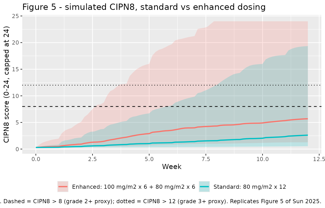
peak_std <- peak_cipn8(sim_std)
peak_enh <- peak_cipn8(sim_enh)
stopifnot(identical(peak_std$id, peak_enh$id))

# The enhanced regimen doses at least as much as the standard regimen at every
# occasion, so within a subject the gated exposure, the effect compartment and
# hence CIPN8 are all weakly larger. This is a structural monotonicity, not a
# distributional claim, so it must hold for EVERY paired subject.
stopifnot(all(peak_enh$peak >= peak_std$peak - 1e-6))
# The median contrast is the robust distributional statement. No bound is placed
# on either median individually: with omegas this large the cohort median moves
# substantially between random draws (see Errata).
stopifnot(stats::median(peak_enh$peak) > stats::median(peak_std$peak))
External evaluation: grade 3+ CIPN incidence
Results 3.2 compares simulated grade 3+ incidence (CIPN8 > 12 at any time) against the rates reported by CALGB C9840. The table reproduces that comparison from the packaged model.
incidence <- dplyr::bind_rows(
  dplyr::mutate(peak_std, arm = "Standard (80 mg/m2 x 12)"),
  dplyr::mutate(peak_enh, arm = "Enhanced (100 x 6 + 80 x 6)")
) |>
  dplyr::group_by(.data$arm) |>
  dplyr::summarise(
    `Simulated here, CIPN8 > 12 (%)` = 100 * mean(.data$peak > 12),
    `Median peak CIPN8` = stats::median(.data$peak),
    .groups = "drop"
  ) |>
  dplyr::mutate(
    `Sun 2025 simulated (%)` = c(35, 18),
    `C9840 observed (%)` = c(30, 21)
  ) |>
  dplyr::relocate("arm")

knitr::kable(incidence, digits = c(0, 1, 2, 0, 0),
             caption = paste("Grade 3+ CIPN incidence. The 'simulated here'",
                             "column draws a fresh cohort from the population",
                             "model and is expected to exceed the paper's own",
"figures; see Errata."))| arm | Simulated here, CIPN8 > 12 (%) | Median peak CIPN8 | Sun 2025 simulated (%) | C9840 observed (%) |
|---|---|---|---|---|
| Enhanced (100 x 6 + 80 x 6) | 43.0 | 6.47 | 35 | 30 |
| Standard (80 mg/m2 x 12) | 34.5 | 3.90 | 18 | 21 |
# The ordering of the paper's own simulated and observed incidences is the
# reproducible claim; the absolute level from a fresh population draw is not.
stopifnot(all(incidence$`Simulated here, CIPN8 > 12 (%)` > 0))
The fresh-cohort incidences are roughly 30-35% in both arms, well above the paper’s 18% (standard) and 35% (enhanced). This is not a transcription error: it follows directly from the reported shrinkage, and is discussed in the Errata below. The reproducible statements are the within-subject monotonicity and the median contrast asserted above, not the absolute tail incidence.
Assumptions and deviations
Errata and interpretation notes
-
ke0is dimensionally inconsistent as published, and is applied verbatim. Equation 3 readsd ce/dt = cact * ke0withcactin ng/mL and Table 2 labellingke0_popin mL/ng, which makes the right-hand side dimensionless rather than a rate; Table 2’s footnote then labels the effect compartment itself in ng/mL. These three labels cannot all be right. The model reproduces the equation and the value exactly as printed, on the paper’s hour time axis, and the resulting effect-compartment magnitude is verified above against the paper’s own reported 1.56 (agreement about 2%), which is the strongest available evidence that the intended arithmetic has been recovered. The registered canonicalke0is retained because the paper uses that symbol and the parameter plays the effect-compartment linkage role; the divergence from the usualke0 * (Cc - Ce)equilibration form is recorded in theke0entry ofinst/references/parameter-names.md. -
koutunits are inferred. Table 2 printskout_pop = 0.0027with no unit. The PK panel of the same table is in L/hour and the PD model shares that time axis, sokoutis taken as 1/h. This gives a CIPN8 resolution half-life oflog(2)/0.0027= about 257 h (10.7 days), which is consistent with the Discussion’s description of gradual resolution between doses; a 1/day reading would imply a 257-day half-life, which is not. -
cthresis a new canonical registered with this extraction. The paper’s threshold is calledx. No concentration-threshold gate existed in the register:thresis scoped to receptor occupancy (a percent) andmicis a measured pathogen susceptibility, not an estimated PD parameter.cthreswas ratified as an explicit sibling ofthres, with the leadingcmarking that the gated quantity is a concentration. Seeinst/references/parameter-names.md. -
powExp_cipn8 = 0.74is treated as fixed. The exponent appears only inside Table 2’s printed error expression and is absent from the table’s estimated-parameter rows, each of which carries an SE and RSE. It is therefore encoded asfixed(0.74)rather than as an estimated parameter. -
lrbaseis fixed atlog(0.3). Table 2 reportsR0_pop = 0.3with SE and RSE bothNA, and 0.3 is exactly the Table 1 mean baseline CIPN8, so the baseline was held rather than estimated. -
The PD residual error uses
combined1(). Table 2’s footnote givesCIPN8 = R + (a1 + b1 x R^0.74) x e, i.e. the residual SD is a linear sum of an additive and a power term. nlmixr2’s default foradd() + pow()is the root-sum-of-squares form, socombined1()is required to match the printed expression. -
A fresh population draw over-predicts the published CIPN
incidence. The PD omegas are very large on the log scale
(
Omega_kout2.45,Omega_k1.91,Omega_ke00.85) and Table 2 reports their shrinkage as -75%, 52% and 90% respectively. The paper’s 18% and 35% figures come from re-simulating its own 60 patients using their individual parameter estimates, which with 52-90% shrinkage are pulled far toward the population typical value. Drawing a fresh cohort from the population model instead samples the full marginal variance, which is much wider, so the tails are heavier and roughly 20-28% of simulated subjects saturate the 0-24 scale in both arms. Two further contributors push the same way: every simulated subject here receives all 12 doses, whereas the cohort received a mean of 11 (range 3-12) with dose delays and reductions; and the paper itself notes the PD shrinkage is “slightly negative (-0.08), indicating potential overfitting”. Downstream users who want to reproduce the paper’s incidence figures should condition on individual parameters rather than sample from the population model. -
The 18-26 h concentration reads low at typical
values (about 15 ng/mL at 22 h versus a published cohort mean
of 22.02 ng/mL, inside the observed range of 10-51.80). Two reasons: the
constant residual error is 9.11 ng/mL, which is of the same order as the
concentrations in this window, so those observations carry little weight
in the fit; and with a log-normal
Omega_V1of 0.51 the cohort’s arithmetic mean sits well above the typical-value prediction. The published mean also pools samples drawn anywhere from 16 to 26 h, over which the model’s typical profile falls from about 21 to 12 ng/mL. - Cmax sampling. The observed Cmax was drawn “during the final 10 min before the end of infusion” (Methods 2.1), i.e. slightly before the true end-of-infusion peak, so the published mean is a marginally low estimate of the modelled Cmax. The 1% agreement reported above is therefore if anything conservative.
Assumptions made because the paper does not specify
- BSA distribution. Only the mean cumulative dose and the dose per m2 are reported, from which a cohort mean BSA of 1.838 m2 is derived (Table 1). The spread is assumed normal with SD 0.20 m2 truncated to 1.3-2.5 m2. This affects only the spread of administered doses, not any model parameter.
- All 12 doses administered on schedule. Real dosing histories included delays and reductions (mean 11 of 12 doses received), which were abstracted from the medical record and are not published per patient.
-
No covariate effects. Table 2 reports no covariate
terms and neither Methods 2.2 nor 2.4 describes a covariate search, so
covariateDatais empty. BSA enters only through the administered dose amount. - IIV correlations. Table 2 reports omegas as independent standard deviations with no correlation matrix, so the etas are encoded as uncorrelated.
Scope limitation carried from the paper. The Discussion states the model “should not be directly applied to other paclitaxel regimens without tuning parameters”, having dramatically overestimated CIPN for every-3-week 175 mg/m2 dosing, and that the cohort was entirely female, 93% White, with breast cancer on a weekly regimen.