Gentamicin (Paioni 2021)

Model and source

• Citation: Paioni P, Jaggi VF, Tilen R, Seiler M, Baumann P, Bram DS, Jetzer C, Haid RTU, Goetschi AN, Goers R, Muller D, Coman Schmid D, Meyer zu Schwabedissen HE, Rinn B, Berger C, Kramer SD. Gentamicin Population Pharmacokinetics in Pediatric Patients-A Prospective Study with Data Analysis Using the saemix Package in R. Pharmaceutics. 2021;13(10):1596. doi:10.3390/pharmaceutics13101596.
• Article: https://doi.org/10.3390/pharmaceutics13101596 (open access)
• The online supplement holds figures, the research plan and the start-value ranges of the multistart fit (Table S1); every value used below comes from the main article text, equations and tables. No correction notice was found for this article as of 2026-09-29.

Population

Paioni 2021 is a prospective observational study at University Children’s Hospital Zurich (1 October 2017 to 30 April 2019). It enrolled 109 children aged 0.9 days to 14.5 years (median 29.1 days) receiving gentamicin for at least 48 h; 67 were male and 42 female. Median body weight was 4.23 kg (range 2.5-35, mean 5.42), median gestational age 39.3 weeks (29-42; 11 born before 37 weeks). Serum creatinine was below the 27 umol/L reporting limit in 73 of 107 patients (range < 27-72 umol/L) and median serum urea was 3.20 mmol/L (< 1.8 to 17.3) (Table 1). Indications were suspected (43), suspected superimposed (14) and proven (51) bacterial infection, plus one surgical prophylaxis (Table 2). Patients with cystic fibrosis or on any dialysis / haemofiltration were excluded.

Gentamicin was given once daily per hospital practice (5 mg/kg at age < 7 days, 7.5 mg/kg at >= 7 days) as a 2-min or 30-min infusion. Up to three samples were taken per dosing interval (trough, about 30 min and about 4 h after the end of the second or third infusion): 310 concentrations, 71 below the 0.3 mg/L LOQ.

The same information is available programmatically via readModelDb("Paioni_2021_gentamicin")()$population.

Source trace

Equation / parameter	Value	Source location
Two-compartment model, zero-order infusion, linear distribution and elimination	n/a	Section 2.3, Equations (1)-(5); Section 3.2
lambda_z = CL / (V1 + V2')	n/a	Section 2.3 text following Equation (1)
f1 = (1/V1) * (k21 - lambda1)/(lambda_z - lambda1) * CL/lambda1	n/a	Equation (2)
k21 = lambda1 * lambda_z * V1 / CL	n/a	Equation (3)
Covariate equations (power of cov / ref)	n/a	Table 3 equation rows
lcl	2.267 (ln L/d)	Table 3, q1
lvparea (V2’)	-0.174 (ln L)	Table 3, q2
lalpha (lambda1)	3.644 (ln 1/d)	Table 3, q3
lvc (V1)	0.204 (ln L)	Table 3, q4
e_wt_cl	1.219	Table 3, q5 (reference ln(4 kg))
e_creat_cl	-0.964	Table 3, q6 (reference ln(27 uM))
e_bun_cl	-0.168	Table 3, q7 (reference ln(3 mM))
e_wt_vparea	0.974	Table 3, q8 (reference ln(4 kg))
e_wt_vc	0.688	Table 3, q9 (reference ln(4 kg))
etalcl	0.107 (variance)	Table 3, variance of random effects ln(CL)
etalvparea	0.291 (variance)	Table 3, variance of random effects ln(V2’)
etalvc	0.0391 (variance)	Table 3, variance of random effects ln(V1)
No IIV on lambda1	n/a	Sections 3.2 and 3.3
expSd	0.102	Table 3, residual error; “exponential” error model, Section 2.3

Parameterisation

The authors fit the closed-form bi-exponential solution (Equation 1) with four parameters: CL, the central volume V1, the fast disposition rate constant lambda1, and an apparent peripheral volume V2’ defined so that the terminal rate constant is lambda_z = CL / (V1 + V2’). V1 + V2’ is therefore the terminal-phase volume (V_z, “V_area”), not the steady-state volume, and V2’ is not the peripheral volume of the micro-constant parameterisation. The packaged model keeps the authors’ four parameters (so every ini() value appears in Table 3) and derives the micro-constants from the two-compartment identities

• kel = CL / V1
• k21 = lambda1 * lambda_z / kel (Equation 3)
• k12 = lambda1 + lambda_z - kel - k21

The derived peripheral volume vp = V1 * k12 / k21 and inter-compartmental clearance q = k12 * V1 are carried as model outputs. For the typical 4-kg patient, V2’ = 0.840 L while the micro-constant peripheral volume is 0.667 L.

The chunk below checks that the ODE model reproduces the paper’s closed form (Equations 1, 2, 4 and 5) for a typical patient given three 30-min infusions. Both sides use the same parameters, so the agreement is limited only by the ODE solver tolerance.

mod <- readModelDb("Paioni_2021_gentamicin")
mod_typ <- rxode2::zeroRe(mod)
#> ℹ parameter labels from comments will be replaced by 'label()'

typ_cov <- data.frame(WT = 4, CREAT = 27, BUN = 3)
dose_mg <- 7.5 * typ_cov$WT
tinf <- 0.5
obs_t <- sort(unique(c(seq(0, 72, by = 0.25), 48 + tinf + 0.5)))

ev_typ <- dplyr::bind_rows(
  data.frame(time = c(0, 24, 48), evid = 1, amt = dose_mg, dur = tinf, cmt = "central"),
  data.frame(time = obs_t, evid = 0, amt = 0, dur = 0, cmt = "central")
) |>
  dplyr::mutate(id = 1L, WT = typ_cov$WT, CREAT = typ_cov$CREAT, BUN = typ_cov$BUN) |>
  dplyr::arrange(time, dplyr::desc(evid))

sim_typ <- rxode2::rxSolve(mod_typ, events = ev_typ, returnType = "data.frame")
#> ℹ omega/sigma items treated as zero: 'etalcl', 'etalvparea', 'etalvc'

# Paper Equation (1), time in hours. Parameters from Table 3 at the reference
# covariates, converted from per-day to per-hour.
cl <- exp(2.267) / 24
v1 <- exp(0.204)
v2a <- exp(-0.174)
l1 <- exp(3.644) / 24
lz <- cl / (v1 + v2a)
k21 <- l1 * lz * v1 / cl
f1 <- (1 / v1) * (k21 - l1) / (lz - l1) * cl / l1
r0 <- dose_mg / tinf
closed_form <- function(t) {
  out <- 0
  for (t0 in c(0, 24, 48)) {
    tin <- (t - t0) * ((t - t0) <= tinf) * ((t - t0) >= 0)
    tel <- (t - t0 - tinf) * ((t - t0 - tinf) >= 0)
    after <- (tinf + t0) < t
    term <- function(lam) {
      (1 - exp(-lam * tin)) + (1 - exp(-lam * tinf)) * exp(-lam * tel) * after
    }
    out <- out + r0 / cl * (f1 * term(l1) + (1 - f1) * term(lz))
  }
  out
}

chk <- sim_typ |>
  dplyr::filter(time > 0) |>
  dplyr::mutate(Cc_eq1 = closed_form(time), rel_diff = (Cc - Cc_eq1) / Cc_eq1)

c(f1 = f1, max_abs_rel_diff = max(abs(chk$rel_diff)))
#>               f1 max_abs_rel_diff 
#>     9.530452e-02     4.451086e-07
stopifnot(max(abs(chk$rel_diff)) < 1e-3)

Virtual cohort

The individual data are not public (they are held on the SPHN Leonhard Med platform). The simulations below draw a virtual cohort whose covariate distributions approximate Table 1:

• body weight: log-normal with location log(3.0 kg) and log-SD 0.7, truncated to the observed 2.5-35 kg range (after truncation this gives a median of about 4.3 kg and a mean of about 5.3 kg, against 4.23 and 5.42 kg in Table 1);
• serum creatinine: 68% (73/107) at the 27 umol/L reporting limit, the rest log-uniform between 27 and 72 umol/L;
• serum urea: log-normal, median 3.2 mmol/L and log-SD 0.45, truncated to 1.8-17.3 mmol/L.

Covariates are drawn independently; the paper does not report their joint distribution.

set.seed(20211001)
n_per_arm <- 200L

draw_trunc_lnorm <- function(n, meanlog, sdlog, lo, hi) {
  out <- numeric(0)
  while (length(out) < n) {
    x <- rlnorm(n, meanlog, sdlog)
    out <- c(out, x[x >= lo & x <= hi])
  }
  out[seq_len(n)]
}

make_covariates <- function(n) {
  creat_censored <- runif(n) < 73 / 107
  data.frame(
    WT = draw_trunc_lnorm(n, log(3.0), 0.7, 2.5, 35),
    CREAT = ifelse(creat_censored, 27, exp(runif(n, log(27), log(72)))),
    BUN = draw_trunc_lnorm(n, log(3.2), 0.45, 1.8, 17.3)
  )
}

covs <- make_covariates(n_per_arm)
summary(covs)
#>        WT             CREAT            BUN        
#>  Min.   : 2.506   Min.   :27.00   Min.   : 1.826  
#>  1st Qu.: 3.276   1st Qu.:27.00   1st Qu.: 2.593  
#>  Median : 4.148   Median :27.00   Median : 3.341  
#>  Mean   : 5.156   Mean   :32.34   Mean   : 3.666  
#>  3rd Qu.: 6.033   3rd Qu.:30.52   3rd Qu.: 4.160  
#>  Max.   :16.995   Max.   :71.60   Max.   :11.941

Typical-value PK parameters across the cohort (Table 4)

Table 4 of the paper summarises the population-level (covariate-only) PK parameters of the 109 study patients. The same quantities computed for the virtual cohort:

pk_typ <- covs |>
  dplyr::mutate(
    cl_Lh = exp(2.267 + 1.219 * log(WT / 4) - 0.964 * log(CREAT / 27) - 0.168 * log(BUN / 3)) / 24,
    v1 = exp(0.204 + 0.688 * log(WT / 4)),
    v2a = exp(-0.174 + 0.974 * log(WT / 4)),
    vz = v1 + v2a,
    CL_mLmin = cl_Lh * 1000 / 60,
    t_half = log(2) * vz / cl_Lh
  )

tab4 <- tibble::tribble(
  ~parameter, ~published_median, ~published_range,
  "CL (mL/min)", 6.88, "2.76-73.2",
  "Vz = V1 + V2' (L)", 2.16, "1.42-12.4",
  "V1 (L)", 1.27, "0.887-5.46",
  "t1/2 (h)", 3.53, "1.72-8.38"
) |>
  dplyr::mutate(
    simulated_median = c(
      median(pk_typ$CL_mLmin), median(pk_typ$vz),
      median(pk_typ$v1), median(pk_typ$t_half)
    ),
    simulated_range = c(
      paste(signif(range(pk_typ$CL_mLmin), 3), collapse = "-"),
      paste(signif(range(pk_typ$vz), 3), collapse = "-"),
      paste(signif(range(pk_typ$v1), 3), collapse = "-"),
      paste(signif(range(pk_typ$t_half), 3), collapse = "-")
    ),
    pct_diff = 100 * (simulated_median - published_median) / published_median
  )

tab4 |>
  dplyr::rename(
    "Parameter" = parameter,
    "Published median" = published_median,
    "Published range" = published_range,
    "Virtual-cohort median" = simulated_median,
    "Virtual-cohort range" = simulated_range,
    "% difference of medians" = pct_diff
  ) |>
  knitr::kable(digits = 2, caption = "Population-level PK parameters: Table 4 of Paioni 2021 vs the virtual cohort.")

Population-level PK parameters: Table 4 of Paioni 2021 vs the virtual cohort.

Parameter	Published median	Published range	Virtual-cohort median	Virtual-cohort range	% difference of medians
CL (mL/min)	6.88	2.76-73.2	6.36	1.64-38.1	-7.55
Vz = V1 + V2’ (L)	2.16	1.42-12.4	2.13	1.42-6.76	-1.49
V1 (L)	1.27	0.887-5.46	1.26	0.889-3.32	-1.00
t1/2 (h)	3.53	1.72-8.38	3.86	1.97-10.8	9.47

# Structural check on the medians: a mis-transcribed intercept or exponent
# moves these by tens of percent. Weight is the dominant covariate and the
# virtual cohort matches the Table 1 weight median only approximately.
stopifnot(all(abs(tab4$pct_diff) < 10))

Scale of the Table 3 random effects

Table 3 labels the inter-individual terms “Variance of the random effects”, the quantity saemix reports. Table 4 independently confirms that reading: it prints each PK parameter at the population level (covariates only) and at the individual level (covariates plus the fitted random effects), and the gap between the two extremes fixes a minimum size for the random effect of at least one patient. Population-level V1 per 70 kg is largest at the lightest weight (2.5 kg), where the model gives the Table 4 value of 24.8 L/70 kg, yet one patient’s individual V1 reaches 33.4 L/70 kg. Likewise the lowest individual CL is 19.7 mL/min per 70 kg against a population-level minimum of 42.4.

v1_70_max <- exp(0.204) * (2.5 / 4)^0.688 * 70 / 2.5
eta_v1_min <- log(33.4 / 24.8)
eta_cl_min <- log(19.7 / 42.4)
omega_check <- tibble::tibble(
  parameter = c("V1", "CL"),
  printed_value = c(0.0391, 0.107),
  min_abs_eta = abs(c(eta_v1_min, eta_cl_min))
) |>
  dplyr::mutate(
    z_if_variance = min_abs_eta / sqrt(printed_value),
    z_if_sd = min_abs_eta / printed_value
  )
omega_check |>
  dplyr::rename(
    "Parameter" = parameter,
    "Table 3 value" = printed_value,
    "Smallest |eta| implied by Table 4" = min_abs_eta,
    "|eta| / SD, value read as variance" = z_if_variance,
    "|eta| / SD, value read as SD" = z_if_sd
  ) |>
  knitr::kable(digits = 2, caption = "Random-effect size implied by the Table 4 individual-level extremes.")

Random-effect size implied by the Table 4 individual-level extremes.

Parameter	Table 3 value	Smallest |eta| implied by Table 4	|eta| / SD, value read as variance	|eta| / SD, value read as SD
V1	0.04	0.30	1.51	7.61
CL	0.11	0.77	2.34	7.16

# Deterministic (no cohort): the population-level bound reproduces Table 4, and
# only the variance reading keeps the implied random effects plausible.
stopifnot(
  abs(v1_70_max / 24.8 - 1) < 0.01,
  all(omega_check$z_if_variance < 3),
  all(omega_check$z_if_sd > 5)
)

Read as SDs, the printed values would require random effects of 7 or more standard deviations, so the model encodes them as variances.

Simulation of the typical once-daily regimens (Figure 7)

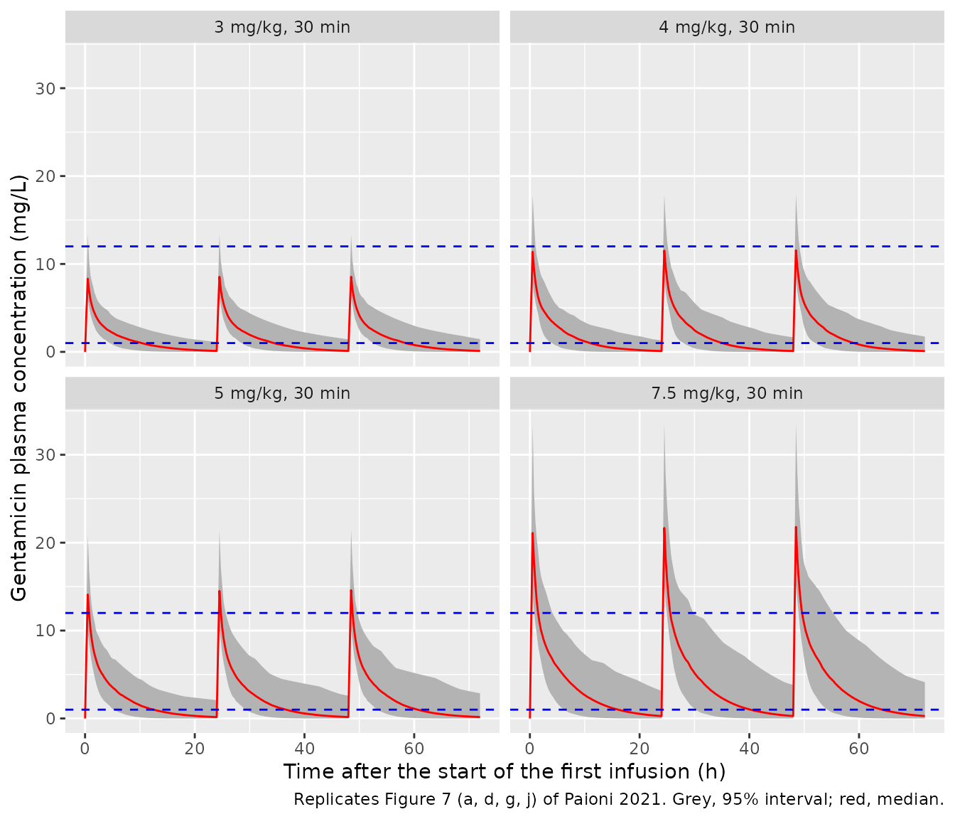
Section 3.7 simulates three 24-hourly doses of 3, 4, 5 and 7.5 mg/kg in the study population with the random effects of Table 3 and no residual error, and reports the 95% interval of the concentration 30 min after the end of the third infusion, C(30 min’). The virtual cohort above is dosed with each regimen as a 30-min infusion, and with 7.5 mg/kg as a 2-min infusion.

regimens <- tibble::tribble(
  ~regimen, ~mgkg, ~tinf,
  "3 mg/kg, 30 min", 3, 0.5,
  "4 mg/kg, 30 min", 4, 0.5,
  "5 mg/kg, 30 min", 5, 0.5,
  "7.5 mg/kg, 30 min", 7.5, 0.5,
  "7.5 mg/kg, 2 min", 7.5, 2 / 60
)

make_arm <- function(i, covs) {
  r <- regimens[i, ]
  n <- nrow(covs)
  ids <- (i - 1L) * n + seq_len(n)
  obs_t <- sort(unique(c(seq(0, 72, by = 0.25), 48 + r$tinf + 0.5, 72)))
  subj <- covs |> dplyr::mutate(id = ids, regimen = r$regimen)
  doses <- subj |>
    tidyr::crossing(time = c(0, 24, 48)) |>
    dplyr::mutate(evid = 1L, amt = r$mgkg * WT, dur = r$tinf, cmt = "central")
  obs <- subj |>
    tidyr::crossing(time = obs_t) |>
    dplyr::mutate(evid = 0L, amt = 0, dur = 0, cmt = "central")
  dplyr::bind_rows(doses, obs)
}

events <- dplyr::bind_rows(lapply(seq_len(nrow(regimens)), make_arm, covs = covs)) |>
  dplyr::arrange(id, time, dplyr::desc(evid))
stopifnot(!anyDuplicated(unique(events[, c("id", "time", "evid")])))

rxode2::rxSetSeed(20211001)
sim <- rxode2::rxSolve(mod, events = events, keep = c("regimen", "WT"), returnType = "data.frame") |>
  dplyr::mutate(regimen = factor(regimen, levels = regimens$regimen))
#> ℹ parameter labels from comments will be replaced by 'label()'

# Sensitivity run: the Table 3 values used as standard deviations (so each
# variance is the square of the printed value). See "C(30 min') after the
# third dose" below for why.
mod_sd <- mod |>
  rxode2::ini(etalcl ~ 0.011449, etalvparea ~ 0.084681, etalvc ~ 0.00152881)
#> ℹ parameter labels from comments will be replaced by 'label()'
#> ℹ change initial estimate of `etalcl` to `0.011449`
#> ℹ change initial estimate of `etalvparea` to `0.084681`
#> ℹ change initial estimate of `etalvc` to `0.00152881`
rxode2::rxSetSeed(20211001)
sim_sd <- rxode2::rxSolve(mod_sd, events = events, keep = c("regimen", "WT"), returnType = "data.frame") |>
  dplyr::mutate(regimen = factor(regimen, levels = regimens$regimen))

# Replicates Figure 7 (a, d, g, j) of Paioni 2021: 95% interval and median of
# the simulated concentration-time curves for 30-min infusions.
sim |>
  dplyr::filter(grepl("30 min", regimen)) |>
  dplyr::group_by(regimen, time) |>
  dplyr::summarise(
    lo = quantile(Cc, 0.025), med = median(Cc), hi = quantile(Cc, 0.975),
    .groups = "drop"
  ) |>
  ggplot(aes(time, med)) +
  geom_ribbon(aes(ymin = lo, ymax = hi), fill = "grey70") +
  geom_line(colour = "red") +
  geom_hline(yintercept = c(1, 12), colour = "blue", linetype = "dashed") +
  facet_wrap(~regimen) +
  labs(
    x = "Time after the start of the first infusion (h)",
    y = "Gentamicin plasma concentration (mg/L)",
    caption = "Replicates Figure 7 (a, d, g, j) of Paioni 2021. Grey, 95% interval; red, median."
  )

C(30 min’) after the third dose

summarise_c30 <- function(s, label) {
  s |>
    dplyr::mutate(t30 = 48 + regimens$tinf[match(as.character(regimen), regimens$regimen)] + 0.5) |>
    dplyr::filter(abs(time - t30) < 1e-6) |>
    dplyr::group_by(regimen) |>
    dplyr::summarise(
      sim_lo = quantile(Cc, 0.025), sim_med = median(Cc), sim_hi = quantile(Cc, 0.975),
      .groups = "drop"
    ) |>
    dplyr::mutate(iiv = label)
}
c30 <- dplyr::bind_rows(
  summarise_c30(sim, "Table 3 as variances (packaged model)"),
  summarise_c30(sim_sd, "Table 3 as SDs (sensitivity)")
)

pub_c30 <- tibble::tribble(
  ~regimen, ~pub_lo, ~pub_hi,
  "3 mg/kg, 30 min", 5.2, 8.4,
  "4 mg/kg, 30 min", 6.9, 11.3,
  "5 mg/kg, 30 min", NA, NA,
  "7.5 mg/kg, 30 min", 13.0, 21.2,
  "7.5 mg/kg, 2 min", 14.6, 25.0
)

c30_cmp <- c30 |>
  dplyr::mutate(regimen = as.character(regimen)) |>
  dplyr::left_join(pub_c30, by = "regimen") |>
  dplyr::mutate(
    pub_mid = sqrt(pub_lo * pub_hi),
    pct_diff_mid = 100 * (sim_med - pub_mid) / pub_mid
  )

c30_cmp |>
  dplyr::select(iiv, regimen, pub_lo, pub_hi, sim_lo, sim_med, sim_hi, pct_diff_mid) |>
  dplyr::rename(
    "IIV" = iiv,
    "Regimen" = regimen,
    "Published 2.5%" = pub_lo,
    "Published 97.5%" = pub_hi,
    "Simulated 2.5%" = sim_lo,
    "Simulated median" = sim_med,
    "Simulated 97.5%" = sim_hi,
    "% diff of median vs published interval midpoint" = pct_diff_mid
  ) |>
  knitr::kable(digits = 1, caption = "C(30 min') after the third dose (mg/L): Section 3.7 of Paioni 2021 vs simulation.")

C(30 min’) after the third dose (mg/L): Section 3.7 of Paioni 2021 vs simulation.

IIV	Regimen	Published 2.5%	Published 97.5%	Simulated 2.5%	Simulated median	Simulated 97.5%	% diff of median vs published interval midpoint
Table 3 as variances (packaged model)	3 mg/kg, 30 min	5.2	8.4	4.3	6.2	9.2	-6.4
Table 3 as variances (packaged model)	4 mg/kg, 30 min	6.9	11.3	5.8	8.3	12.7	-5.8
Table 3 as variances (packaged model)	5 mg/kg, 30 min	NA	NA	7.4	10.4	15.2	NA
Table 3 as variances (packaged model)	7.5 mg/kg, 30 min	13.0	21.2	11.8	15.9	24.4	-4.4
Table 3 as variances (packaged model)	7.5 mg/kg, 2 min	14.6	25.0	13.2	17.9	27.2	-6.5
Table 3 as SDs (sensitivity)	3 mg/kg, 30 min	5.2	8.4	5.3	6.2	8.2	-5.8
Table 3 as SDs (sensitivity)	4 mg/kg, 30 min	6.9	11.3	7.0	8.3	10.7	-6.3
Table 3 as SDs (sensitivity)	5 mg/kg, 30 min	NA	NA	8.8	10.4	13.3	NA
Table 3 as SDs (sensitivity)	7.5 mg/kg, 30 min	13.0	21.2	13.3	15.6	20.1	-5.9
Table 3 as SDs (sensitivity)	7.5 mg/kg, 2 min	14.6	25.0	15.3	17.7	22.4	-7.3

# The paper does not print the median, so the centre is compared with the
# geometric midpoint of the published 95% interval. A mis-transcribed volume or
# clearance moves this by tens of percent.
stopifnot(all(abs(c30_cmp$pct_diff_mid) < 12, na.rm = TRUE))

The centre of every published interval is reproduced. The published intervals are, however, markedly narrower than those of the packaged model (for example 5.2-8.4 mg/L at 3 mg/kg), and they are matched closely when the Table 3 values are used as standard deviations instead of variances. The Table 4 check above shows the fitted random effects are variances, so the paper’s own Section 3.7 simulations appear to have drawn the random effects with the printed variance used as the standard deviation (Section 2.7 describes drawing from N(0, s^2) “with s equal the standard deviation of the respective random effect”). The packaged model keeps the fitted variances; its C(30 min’) and C(24 h’) intervals are therefore wider than those printed in the paper. The paper also reports the 99% interval of C(30 min’) at 5 mg/kg (8.2-16.9 mg/L) and at 7.5 mg/kg (12.4-25.4 mg/L), both for 30-min infusions (Discussion).

# Section 3.7 / Discussion: for doses up to 4 mg/kg, >= 95% of simulated
# C(24 h') (24 h after the start of the third infusion) were below 1 mg/L;
# abstract: at 7.5 mg/kg 95% were < 1.8 mg/L.
summarise_c24 <- function(s, label) {
  s |>
    dplyr::filter(time == 72) |>
    dplyr::group_by(regimen) |>
    dplyr::summarise(
      q95 = quantile(Cc, 0.95),
      pct_below_1 = 100 * mean(Cc < 1),
      .groups = "drop"
    ) |>
    dplyr::mutate(iiv = label, .before = 1)
}
c24 <- dplyr::bind_rows(
  summarise_c24(sim, "Table 3 as variances (packaged model)"),
  summarise_c24(sim_sd, "Table 3 as SDs (sensitivity)")
)
c24 |>
  dplyr::rename(
    "IIV" = iiv,
    "Regimen" = regimen,
    "95th percentile (mg/L)" = q95,
    "% below 1 mg/L" = pct_below_1
  ) |>
  knitr::kable(digits = 2, caption = "Simulated C(24 h') after the third dose.")

Simulated C(24 h’) after the third dose.

IIV	Regimen	95th percentile (mg/L)	% below 1 mg/L
Table 3 as variances (packaged model)	3 mg/kg, 30 min	1.08	94.5
Table 3 as variances (packaged model)	4 mg/kg, 30 min	1.26	93.5
Table 3 as variances (packaged model)	5 mg/kg, 30 min	1.89	89.0
Table 3 as variances (packaged model)	7.5 mg/kg, 30 min	3.31	76.5
Table 3 as variances (packaged model)	7.5 mg/kg, 2 min	2.53	82.5
Table 3 as SDs (sensitivity)	3 mg/kg, 30 min	0.68	98.0
Table 3 as SDs (sensitivity)	4 mg/kg, 30 min	0.89	96.5
Table 3 as SDs (sensitivity)	5 mg/kg, 30 min	1.23	92.0
Table 3 as SDs (sensitivity)	7.5 mg/kg, 30 min	1.97	87.0
Table 3 as SDs (sensitivity)	7.5 mg/kg, 2 min	1.79	89.5

PKNCA validation

The paper reports no NCA table. Its Table 4 gives the median terminal half-life of the study patients at the population level (covariates only, no random effects), 3.53 h. PKNCA is therefore run over the first dosing interval (0-24 h) of each 30-min regimen on a typical-value solve of the virtual cohort (random effects set to zero), which is the same quantity.

ev_30 <- events |> dplyr::filter(grepl("30 min", regimen))
# rxode2 warns that a multi-subject solve has no omega; that is the intent here.
sim_pop <- suppressWarnings(
  rxode2::rxSolve(mod_typ, events = ev_30, keep = c("regimen"), returnType = "data.frame")
)
#> ℹ omega/sigma items treated as zero: 'etalcl', 'etalvparea', 'etalvc'

sim_nca <- sim_pop |>
  dplyr::filter(!is.na(Cc)) |>
  dplyr::mutate(regimen = as.character(regimen)) |>
  dplyr::select(id, time, Cc, regimen)

sim_nca <- dplyr::bind_rows(
  sim_nca,
  sim_nca |> dplyr::distinct(id, regimen) |> dplyr::mutate(time = 0, Cc = 0)
) |>
  dplyr::distinct(id, regimen, time, .keep_all = TRUE) |>
  dplyr::arrange(id, regimen, time)

dose_df <- ev_30 |>
  dplyr::filter(evid == 1, time == 0) |>
  dplyr::select(id, time, amt, dur, regimen)

conc_obj <- PKNCA::PKNCAconc(sim_nca, Cc ~ time | regimen + id)
dose_obj <- PKNCA::PKNCAdose(dose_df, amt ~ time | regimen + id, route = "intravascular", duration = "dur")
intervals <- data.frame(start = 0, end = 24, cmax = TRUE, tmax = TRUE, auclast = TRUE, half.life = TRUE)
nca_res <- PKNCA::pk.nca(PKNCA::PKNCAdata(conc_obj, dose_obj, intervals = intervals))

published <- tibble::tibble(
  regimen = unique(sim_nca$regimen),
  half.life = 3.53
)

cmp <- nlmixr2lib::ncaComparisonTable(
  simulated = nca_res,
  reference = published,
  by = "regimen",
  units = c(cmax = "mg/L", tmax = "h", auclast = "h*mg/L", half.life = "h"),
  tolerance_pct = 20
)
cmp |>
  knitr::kable(caption = "PKNCA over the first dosing interval vs the Table 4 median half-life. * differs from reference by >20%.")

PKNCA over the first dosing interval vs the Table 4 median half-life. * differs from reference by >20%.

NCA parameter	regimen	Reference	Simulated	% diff
t½ (h)	3 mg/kg, 30 min	3.53	3.85	+9.1%
t½ (h)	4 mg/kg, 30 min	3.53	3.85	+9.1%
t½ (h)	5 mg/kg, 30 min	3.53	3.85	+9.1%
t½ (h)	7.5 mg/kg, 30 min	3.53	3.85	+9.1%

The model is linear, so the half-life does not depend on the dose; the four rows differ only through the dose-proportional grid. The residual difference from 3.53 h reflects the virtual cohort’s covariate mix (Table 4 median weight and creatinine are those of the study patients).

Errata in the source

The paper’s simulated concentration intervals are inconsistent with its own Table 3 random-effect variances. Table 3 labels the random effects “Variance of the random effects (inter-individual variance)”, and the Table 4 individual-level extremes confirm that scale (see “Scale of the Table 3 random effects”). The 95% intervals of C(30 min’) printed in Section 3.7, the abstract and the Discussion (3 mg/kg 5.2-8.4, 4 mg/kg 6.9-11.3, 7.5 mg/kg 13.0-21.2 mg/L) are, however, reproduced only when the printed values are used as standard deviations; with the printed variances the intervals are wider. The medians agree under either reading. The packaged model encodes Table 3 verbatim as variances, because the printed estimates take precedence over the paper’s derived simulations. Its C(30 min’) and C(24 h’) intervals are therefore wider than those published. The SD-scale sensitivity run above shows the published intervals are recovered under the alternative reading.

Assumptions and deviations

• Parameter names. The paper’s apparent peripheral volume V2’ is carried as lvparea / vparea and the distribution-phase rate constant lambda1 as lalpha / alpha; the micro-constants and the micro-constant peripheral volume vp are derived (see “Parameterisation”).
• Units. Table 3 reports CL in L/day and lambda1 in 1/day; the model converts both to hours.
• Residual error. saemix’s “exponential” error model is log(y) = log(f) + a * eps; the Table 3 value 0.102 is taken as the log-scale SD a, the quantity saemix reports, and encoded as lnorm(expSd).
• Censored covariates. Serum creatinine was below the 27 umol/L reporting limit in 73 of 107 patients and the reference value is 27 umol/L; the paper does not say how the censored values were coded. Entering them at 27 umol/L is assumed (and is what the virtual cohort does). Supplying a creatinine below 27 umol/L extrapolates the power effect beyond the data. The coding of the eight urea values below 1.8 mmol/L is also not stated.
• Missing covariates were entered at the reference value in the fit (Section 2.3); do the same when simulating a patient with a missing value.
• Scale of the random effects. Table 3 values are encoded as variances, and the model is not adjusted to reproduce the narrower published simulation intervals; see “Errata in the source”.
• Structural constraint. The fit rejected parameter sets with CL > lambda1 * V1 (Section 2.3). For such a set the derived k12 is negative; the ODE still reproduces the paper’s bi-exponential Equation (1) but the peripheral amount is no longer physical. This only occurs far outside the covariate range of the study (for example a heavy child with a low creatinine and a high CL random effect).
• Virtual cohort. Covariates were drawn independently from distributions matched to the Table 1 summary statistics; the study’s own 109 patients (whom the paper’s simulations used, 100 replicates each) are not available.
• BLQ handling in the fit (Section 2.4) affects estimation only and has no counterpart in the simulation model. The bracketed Table 3 values from the LOQ/2 sensitivity analysis are not used.