Obiltoxaximab animal-to-human dose translation (Nagy 2017)
Source:vignettes/articles/Nagy_2017_obiltoxaximab.Rmd
Nagy_2017_obiltoxaximab.Rmd
library(nlmixr2lib)
library(PKNCA)
#>
#> Attaching package: 'PKNCA'
#> The following object is masked from 'package:stats':
#>
#>     filter
library(rxode2)
#> rxode2 5.1.8 using 2 threads (see ?getRxThreads)
#>   no cache: create with `rxCreateCache()`
library(dplyr)
#>
#> Attaching package: 'dplyr'
#> The following objects are masked from 'package:stats':
#>
#>     filter, lag
#> The following objects are masked from 'package:base':
#>
#>     intersect, setdiff, setequal, union
library(ggplot2)
Overview
Obiltoxaximab is a chimeric IgG1(kappa) monoclonal antibody against anthrax protective antigen (PA). Because human efficacy trials for inhalational anthrax are neither ethical nor feasible, it was approved under the US FDA Animal Rule: efficacy is established in animals and the human dose is justified by comparing exposures. Nagy et al. (2017) is that justification.
Two models come out of the paper and both are extracted here.
-
Nagy_2017_obiltoxaximab– a joint two-compartment population PK model carrying the NZW rabbit, cynomolgus macaque and human parameter sets from Supplementary Table S1 in one file, with first-order intramuscular absorption in animals and a parallel Michaelis-Menten elimination arm approximating PA-mediated target-mediated drug disposition (TMDD) in infected subjects. -
Nagy_2017_obiltoxaximab_survival– the Weibull cure-rate survival model (Supplementary Table S2) that established 16 mg/kg as the efficacious animal dose.
mod <- readModelDb("Nagy_2017_obiltoxaximab")
surv <- readModelDb("Nagy_2017_obiltoxaximab_survival")

# readModelDb() returns the model function; the file-level metadata lives on the
# compiled rxode2 user-interface object.
mod_meta <- rxode2::rxode(mod)$meta
Population
PK data came from ten studies: two in NZW rabbits (one healthy, one infected), five in cynomolgus macaques (one healthy, four infected) and three in healthy human volunteers, giving 791, 929 and 2,830 observations respectively. Healthy and infected animal data were fit simultaneously within each species so the disease effect on PK could be estimated. Animals were challenged with a target 200 LD50 of Bacillus anthracis (Ames strain) spores and treated on a trigger (body-temperature rise in rabbits, positive serum PA signal in macaques). No human anthrax patients were studied: infected-human exposure is a model projection, which is the crux of the Animal Rule argument.
str(mod_meta$population)
#> List of 7
#>  $ species      : chr "human + rabbit (New Zealand White) + cynomolgus macaque"
#>  $ n_subjects   : int 758
#>  $ n_studies    : int 10
#>  $ weight_range : chr "rabbits 2.9-4.0 kg; macaques 2.7-7.3 kg; humans 50-125 kg"
#>  $ disease_state: chr "Pooled healthy and Bacillus anthracis (Ames) aerosol-challenged NZW rabbits and cynomolgus macaques, plus healt"| __truncated__
#>  $ dose_range   : chr "Rabbits: 3, 10, 30 mg/kg i.v. and 10 mg/kg i.m. (healthy); 1, 4, 8, 16 mg/kg i.v. (infected). Macaques: 3, 10, "| __truncated__
#>  $ notes        : chr "n_studies = 10 per Nagy 2017 Methods ('PK data from 10 studies (two studies in rabbits, five studies in macaque"| __truncated__
Source trace
Every equation and every ini() value, with its location
in the source.
| Item | Value | Source |
|---|---|---|
| Two-compartment structure (CL, Vc, Vp, Q), all species | structural | Results, ‘Animal and human population pharmacokinetic modeling’ |
| First-order i.m. absorption (Ka, F1), animals only | structural | Results, same paragraph |
| Parallel Michaelis-Menten arm, infected animals only | structural | Results, same paragraph |
| Macaque nonlinear arm carried to infected humans, allometrically scaled | structural | Methods, ‘Population pharmacokinetic modeling and simulation’ |
| Allometric reference weight, NZW rabbit | 3.165 kg | Results, same paragraph |
| Allometric reference weight, cynomolgus macaque | 2.88 kg | Results, same paragraph |
| Body weight used for all human simulations | 75 kg | Methods, ‘Population pharmacokinetic modeling and simulation’ |
| CL / Vc / Vp / Q, human | 0.233 / 3.21 / 2.73 / 0.473 | Supplementary Table S1, Humans column |
| CL / Vc / Vp / Q, NZW rabbit | 0.0263 / 0.114 / 0.0744 / 0.119 | Supplementary Table S1, NZW Rabbits column |
| CL / Vc / Vp / Q, cynomolgus macaque | 0.0191 / 0.134 / 0.123 / 0.0890 | Supplementary Table S1, Cynomolgus Macaques column |
| Ka / F1, NZW rabbit | 0.961 / 0.899 | Supplementary Table S1 |
| Ka / F1, cynomolgus macaque | 3.89 / 0.895 | Supplementary Table S1 |
| Vmax / Km, NZW rabbit | 0.912 / 10.4 | Supplementary Table S1 |
| Vmax / Km, cynomolgus macaque | 0.275 / 3.21 | Supplementary Table S1 |
| Allometric exponents on CL/Q and Vc/Vp | 0.75 / 1 assumed | not reported; see Assumptions below |
| Survivor function P(T>t) = psurv + (1-psurv)exp(-(lambda t)^alpha) | equation | Results, ‘Animal survival modeling’ |
| logit(psurv) = theta0 - exp((theta1 log10 PTT)^theta2) + Emax dose/(ED50+dose) | equation | Nagy 2017 Results, ‘Animal survival modeling’; exp() printed by Yamamoto 2016 Methods, ‘Survival modeling’ |
| log(lambda) = lambda0 + lambda1 log10 PTT | equation | Results, ‘Animal survival modeling’ |
| theta0 / Emax / ED50 / theta1 | 0.105 / 4.060 / 1.640 / 0.296 | Supplementary Table S2 |
| theta2 / lambda0 / lambda1 / alpha | 1.320 / -2.240 / 0.171 / 2.830 | Supplementary Table S2 |
The three equation blocks were recovered verbatim from the PDF with
pdftotext -layout (page 4, right column). The
exp() around the bacteremia term in
logit(psurv) is taken from the second published report of
this same fitted model, Yamamoto 2016 (doi:10.1128/AAC.00972-16), which prints that equation in
full; see Assumptions and deviations.
Population PK simulation
The paper’s central comparison is a single 16 mg/kg i.v. dose given to each species, healthy and infected. Human doses were infused over 90 minutes; animals received an i.v. bolus.
Supplementary Table S1 reports typical (fixed-effect) values only –
no IIV variances and no residual-error magnitudes are published anywhere
in the paper or its supplements. The model therefore carries
fixed(0) for the residual error and no eta
terms, and every simulation below is a typical-value (deterministic)
profile. Each arm is one subject; there is nothing to average over.
# Observation windows follow the paper's own sampling (Table 1): animals were
# followed to Day 28 post-challenge, humans to Day 71.
arm_spec <- tibble::tribble(
  ~treatment,           ~id, ~wt,   ~rabbit, ~macaque, ~infected, ~dur,     ~tend,
  "Rabbit healthy",     1L,  3.165, 1,       0,        0,         0,        28,
  "Rabbit infected",    2L,  3.165, 1,       0,        1,         0,        28,
  "Macaque healthy",    3L,  2.88,  0,       1,        0,         0,        28,
  "Macaque infected",   4L,  2.88,  0,       1,        1,         0,        28,
  "Human healthy",      5L,  75,    0,       0,        0,         1.5 / 24, 71,
  "Human infected",     6L,  75,    0,       0,        1,         1.5 / 24, 71
)

make_arm <- function(r) {
  # Dense early grid to resolve Cmax, coarser later.
  obs <- unique(c(
    seq(0, 2, by = 0.01),
    seq(2, 10, by = 0.05),
    seq(10, r$tend, by = 0.25)
  ))
  ev <- rxode2::et(amt = 16 * r$wt, dur = r$dur, cmt = "central")
  ev <- rxode2::et(ev, obs)
  d <- as.data.frame(ev)
  # Covariates must be added AFTER materialising to a data frame; assigning
  # onto an rxEt object silently drops them.
  d$id <- r$id
  d$WT <- r$wt
  d$SPECIES_RABBIT <- r$rabbit
  d$SPECIES_MACAQUE <- r$macaque
  d$DIS_ANTHRAX <- r$infected
  d$treatment <- r$treatment
  d
}

events <- dplyr::bind_rows(lapply(seq_len(nrow(arm_spec)), function(i) {
  make_arm(arm_spec[i, ])
}))

sim <- as.data.frame(rxode2::rxSolve(mod, events = events, keep = "treatment"))
#> Warning: multi-subject simulation without without 'omega'
Concentration-time profiles across species
Replicates the comparison in Figure 3 of Nagy 2017 (infected animals versus simulated healthy and infected humans at 16 mg/kg) on the semilogarithmic scale the paper uses in Figure 4.
sim |>
  dplyr::filter(Cc > 1e-3) |>
  ggplot(aes(time, Cc, colour = treatment)) +
  geom_line(linewidth = 0.7) +
  geom_hline(yintercept = c(4.8, 48), linetype = "dashed", colour = "grey40") +
  annotate("text", x = 60, y = 48 * 1.4, label = "99.9% PA neutralization (48 ug/mL)",
           size = 3, colour = "grey30") +
  annotate("text", x = 60, y = 4.8 * 1.4, label = "99% PA neutralization (4.8 ug/mL)",
           size = 3, colour = "grey30") +
  scale_y_log10() +
  labs(x = "Time (days)", y = "Obiltoxaximab concentration (ug/mL)",
       colour = NULL) +
  theme_bw()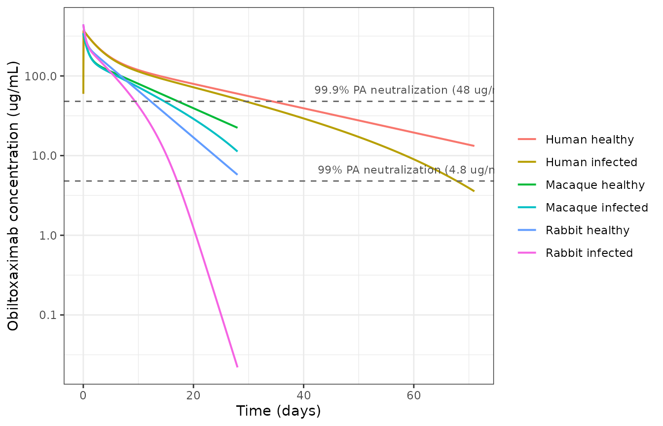
Typical-value obiltoxaximab profiles after a single 16 mg/kg i.v. dose. Replicates the comparison shown in Figures 3 and 4 of Nagy 2017.
The two dashed lines are the concentrations the paper derives for 99%
and 99.9% PA neutralization (4.8 and 48 ug/mL) from
%Bound = 100 * (Kd^-1 * Conc) / (1 + Kd^-1 * Conc) with Kd
= 0.33 nM and MW = 148 kDa (Methods, ‘Neutralization of protective
antigen’). Human concentrations stay above the 99.9% level for roughly
three weeks, which is the paper’s core dose-justification claim.
Noncompartmental analysis
sim_nca <- sim |>
  dplyr::filter(!is.na(Cc)) |>
  dplyr::select(id, time, Cc, treatment)

# Guarantee a time-zero record so PKNCA's AUC interval starts at a measurement.
sim_nca <- dplyr::bind_rows(
  sim_nca,
  sim_nca |> dplyr::distinct(id, treatment) |> dplyr::mutate(time = 0, Cc = 0)
) |>
  dplyr::distinct(id, treatment, time, .keep_all = TRUE) |>
  dplyr::arrange(id, treatment, time)

dose_df <- arm_spec |>
  dplyr::transmute(id, time = 0, amt = 16 * wt, treatment,
                   duration = ifelse(dur == 0, 0, dur))

conc_obj <- PKNCA::PKNCAconc(sim_nca, Cc ~ time | treatment + id,
                             concu = "ug/mL", timeu = "day")
# duration= is required for the infused human arms; without it PKNCA treats the
# dose as an instantaneous bolus and inflates the steady-state volume.
dose_obj <- PKNCA::PKNCAdose(dose_df, amt ~ time | treatment + id,
                             doseu = "mg", duration = "duration")

intervals <- data.frame(
  start = 0, end = Inf,
  cmax = TRUE, tmax = TRUE, aucinf.obs = TRUE,
  half.life = TRUE, cl.obs = TRUE, vss.obs = TRUE
)

nca_res <- PKNCA::pk.nca(PKNCA::PKNCAdata(conc_obj, dose_obj,
                                          intervals = intervals))
Simulated human exposure versus the published simulation (Table 2)
Nagy 2017 Table 2 reports Cmax and AUC0-inf for simulated populations of 500 healthy and 500 infected humans at 16 mg/kg, alongside observed values in infected animals.
published_t2 <- tibble::tribble(
  ~treatment,          ~cmax, ~aucinf.obs,
  "Human healthy",     363,   4980,
  "Human infected",    357,   4070,
  "Macaque infected",  408,   1870,
  "Rabbit infected",   402,   958
)

cmp_t2 <- nlmixr2lib::ncaComparisonTable(
  simulated = nca_res,
  reference = published_t2,
  by = "treatment",
  units = c(cmax = "ug/mL", aucinf.obs = "ug*day/mL"),
  tolerance_pct = 20
)

knitr::kable(
  cmp_t2,
  caption = "Simulated vs. Nagy 2017 Table 2. * differs from reference by >20%.",
  align = c("l", "l", "r", "r", "r")
)| NCA parameter | treatment | Reference | Simulated | % diff |
|---|---|---|---|---|
| Cmax (ug/mL) | Human healthy | 363 | 371 | +2.1% |
| Cmax (ug/mL) | Human infected | 357 | 371 | +3.8% |
| Cmax (ug/mL) | Macaque infected | 408 | 344 | -15.7% |
| Cmax (ug/mL) | Rabbit infected | 402 | 444 | +10.5% |
| AUC0-∞ (obs) (ug*day/mL) | Human healthy | 4980 | 5150 | +3.4% |
| AUC0-∞ (obs) (ug*day/mL) | Human infected | 4070 | 4220 | +3.7% |
| AUC0-∞ (obs) (ug*day/mL) | Macaque infected | 1870 | 1960 | +4.6% |
| AUC0-∞ (obs) (ug*day/mL) | Rabbit infected | 958 | 1440 | +50.1%* |
Cmax reproduces closely in every arm. The two human AUC values sit about 3-4% above the published means, which is expected: the paper’s Table 2 values are means over 500 subjects carrying inter-individual variability, while these are typical-value profiles with IIV fixed to zero (the variances are not published).
One row is starred: infected-rabbit AUC0-inf is 50% above the Table 2 reference of 958 ugday/mL. Infected-macaque AUC agrees to within 5%, so this is specific to the rabbit. The Table 2 animal columns are observed* noncompartmental results, not model predictions, and the infected-rabbit column in particular is a composite mean profile pooling survivors and non-survivors with sampling that stopped 3 days after dosing (Table S3 footnote b; Table 1). Its reported terminal half-life of 1.04 days against 4.17-4.34 days in healthy rabbits from the same table is not a disposition change the population PK model supports. The discrepancy is a property of the published noncompartmental summary rather than of the extracted model; nothing was tuned to close it. See Assumptions and deviations.
The TMDD effect on human exposure
The paper states: “human AUC0-inf is 18% lower when the effects of TMDD are included in the simulation.” This is the single most informative check on the infected-human construction, because it is a ratio and so is insensitive to the missing IIV.
auc_by_arm <- as.data.frame(nca_res$result) |>
  dplyr::filter(PPTESTCD == "aucinf.obs") |>
  dplyr::select(treatment, PPORRES)

auc_healthy <- auc_by_arm$PPORRES[auc_by_arm$treatment == "Human healthy"]
auc_infected <- auc_by_arm$PPORRES[auc_by_arm$treatment == "Human infected"]
pct_drop <- 100 * (1 - auc_infected / auc_healthy)

tibble::tibble(
  Quantity = c("AUC0-inf, healthy human (ug*day/mL)",
               "AUC0-inf, infected human (ug*day/mL)",
               "Reduction attributable to TMDD (%)"),
  Simulated = round(c(auc_healthy, auc_infected, pct_drop), 1),
  Published = c(4980, 4070, 18)
) |>
knitr::kable(caption = "Reproduction of the paper's stated 18% TMDD effect.")| Quantity | Simulated | Published |
|---|---|---|
| AUC0-inf, healthy human (ug*day/mL) | 5147.9 | 4980 |
| AUC0-inf, infected human (ug*day/mL) | 4220.8 | 4070 |
| Reduction attributable to TMDD (%) | 18.0 | 18 |
Animal and human NCA versus the observed data (Tables S3 and S4)
The healthy-animal and human arms can be compared directly against observed noncompartmental results, because those studies had sampling adequate to characterise the terminal phase.
nca_tbl <- as.data.frame(nca_res$result) |>
  dplyr::filter(PPTESTCD %in% c("cl.obs", "vss.obs", "half.life")) |>
  dplyr::select(treatment, PPTESTCD, PPORRES) |>
  tidyr::pivot_wider(names_from = PPTESTCD, values_from = PPORRES)

# Report both absolute and weight-normalised units: Table S4 (human) reports
# CL in L/day and Vss in L, while Table S3 (animals) reports them per kg.
nca_tbl <- nca_tbl |>
  dplyr::left_join(dplyr::select(arm_spec, treatment, wt), by = "treatment") |>
  dplyr::mutate(
    `CL (L/day)` = signif(cl.obs, 3),
    `Vss (L)` = signif(vss.obs, 3),
    `CL (mL/day/kg)` = round(1000 * cl.obs / wt, 2),
    `Vss (mL/kg)` = round(1000 * vss.obs / wt, 1),
    `t1/2 (day)` = round(half.life, 2)
  ) |>
  dplyr::select(Arm = treatment, `CL (L/day)`, `Vss (L)`,
                `CL (mL/day/kg)`, `Vss (mL/kg)`, `t1/2 (day)`)

knitr::kable(
  nca_tbl,
  caption = "Simulated typical-value NCA, in both absolute and weight-normalised units. Observed comparators for the healthy arms -- animals (Table S3, per kg): rabbit CL 8.41-9.22 mL/day/kg, Vss 53.0-58.2 mL/kg, t1/2 4.17-4.34 day; macaque CL 4.18-6.36 mL/day/kg, Vss 67.0-79.4 mL/kg, t1/2 9.36-12.4 day. Human (Table S4, 16 mg/kg, absolute): CL 0.247-0.287 L/day, Vss 5.68-7.18 L, t1/2 19.0-20.4 day."
)| Arm | CL (L/day) | Vss (L) | CL (mL/day/kg) | Vss (mL/kg) | t1/2 (day) |
|---|---|---|---|---|---|
| Human healthy | 0.2330 | 5.940 | 3.11 | 79.2 | 19.62 |
| Human infected | 0.2840 | 4.900 | 3.79 | 65.4 | 7.38 |
| Macaque healthy | 0.0191 | 0.257 | 6.64 | 89.1 | 9.77 |
| Macaque infected | 0.0236 | 0.220 | 8.18 | 76.5 | 5.12 |
| Rabbit healthy | 0.0263 | 0.188 | 8.31 | 59.5 | 5.12 |
| Rabbit infected | 0.0352 | 0.155 | 11.13 | 49.0 | 1.38 |
The healthy arms track the observed data closely. Simulated healthy-rabbit CL is 8.3 mL/day/kg against an observed 8.41-9.22, and healthy-macaque CL is 6.6 mL/day/kg just above an observed 4.18-6.36. For humans the model gives 0.233 L/day and 5.94 L against an observed 0.247-0.287 L/day and 5.68-7.18 L, with a terminal half-life of 19.6 days against an observed 19.0-20.4 days.
The infected arms show the expected direction of the TMDD effect: apparent clearance rises and terminal half-life shortens relative to the healthy arm of the same species, which is the paper’s stated rationale for including the nonlinear arm when projecting infected-human exposure.
The infected-animal arms do not reproduce the observed Table S3 rows, and this is a property of the published NCA rather than of the model – see Assumptions and deviations.
Survival model
The Weibull cure-rate model was fit simultaneously to infected rabbit
and macaque survival data. psurv is the cure fraction
(probability of surviving to the Day-28 end of study) and
lambda is the death rate among the non-cured.
Dose-response by prior-to-treatment bacteremia
Replicates Supplementary Figure S2 of Nagy 2017: predicted survival versus dose, panelled by quartiles of prior-to-treatment (PTT) bacteremia. The published quartile edges are [BLQ, 3.02], [3.03, 3.95], [3.96, 4.87] and (4.87, 8.56] log10 CFU; each curve is evaluated at its quartile midpoint.
quartiles <- tibble::tibble(
  panel = factor(c("[BLQ, 3.02]", "[3.03, 3.95]", "[3.96, 4.87]", "(4.87, 8.56]"),
                 levels = c("[BLQ, 3.02]", "[3.03, 3.95]", "[3.96, 4.87]", "(4.87, 8.56]")),
  ptt = c(2.06, 3.49, 4.42, 6.18)
)

surv_grid <- tidyr::expand_grid(quartiles, dose = seq(0, 32, by = 0.25)) |>
  dplyr::mutate(id = dplyr::row_number())

surv_ev <- surv_grid |>
  dplyr::transmute(id, time = 28,
                   BACT_PTT_LOG10CFU = ptt,
                   DOSE_OBILTOXAXIMAB_MGKG = dose)

surv_sim <- as.data.frame(rxode2::rxSolve(surv, events = surv_ev)) |>
  dplyr::left_join(surv_grid, by = "id")

ggplot(surv_sim, aes(dose, sur)) +
  geom_line(colour = "steelblue", linewidth = 0.8) +
  facet_wrap(~panel) +
  coord_cartesian(ylim = c(0, 1)) +
  labs(x = "Obiltoxaximab dose (mg/kg)",
       y = "Probability of surviving to Day 28") +
  theme_bw()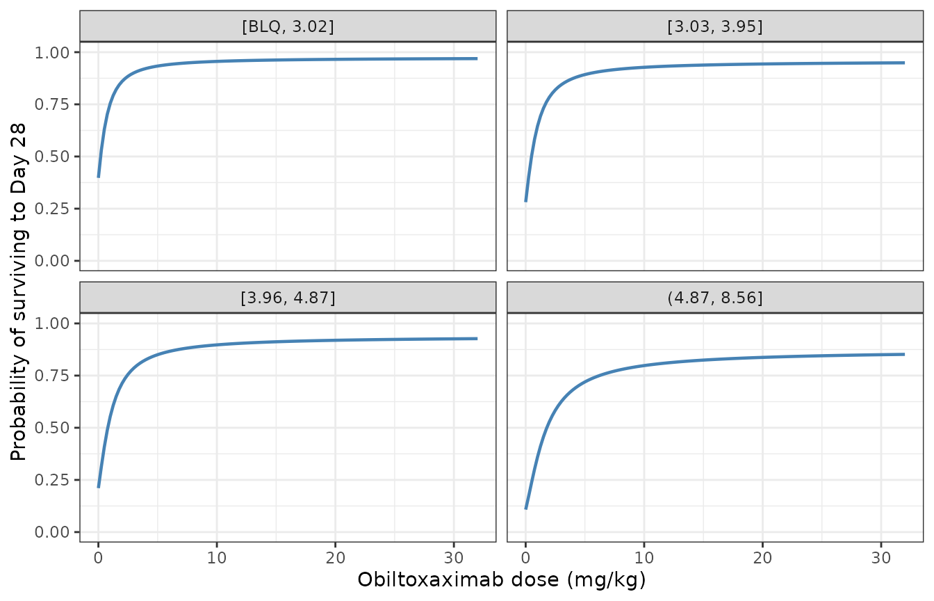
Predicted probability of surviving to Day 28 versus obiltoxaximab dose, by PTT-bacteremia quartile. Replicates Supplementary Figure S2 of Nagy 2017.
ED50, ED90 and the paper’s stated probabilities
Because the dose enters as a plain Emax term, the ED90 is exactly
nine times the ED50 – a closed-form check on the extracted
ed50 and emax.
ed50 <- 1.640
ed90 <- 9 * ed50

tibble::tibble(
  Quantity = c("ED50 (mg/kg)", "ED90 (mg/kg)"),
  Model = round(c(ed50, ed90), 2),
  Published = c(1.64, 14.8)
) |>
knitr::kable(caption = "Dose-response summary against Nagy 2017 Results.")| Quantity | Model | Published |
|---|---|---|
| ED50 (mg/kg) | 1.64 | 1.64 |
| ED90 (mg/kg) | 14.76 | 14.80 |
The paper also states three specific survival probabilities in the
Discussion. psurv_model() below solves the extracted model
itself rather than restating its equation inline, so these checks cannot
silently drift away from the model file the way an earlier revision of
this vignette did (see Assumptions and deviations).
# Evaluate the cure fraction psurv by SOLVING the extracted model. Deliberately
# not a re-typed copy of the logit equation: a hardcoded copy here kept
# "passing" against a dropped exp() in the model file until Yamamoto 2016
# settled the equation form.
psurv_model <- function(dose, ptt) {
  n <- max(length(dose), length(ptt))
  ev <- data.frame(
    id = seq_len(n),
    time = 28,
    BACT_PTT_LOG10CFU = rep_len(ptt, n),
    DOSE_OBILTOXAXIMAB_MGKG = rep_len(dose, n)
  )
  out <- as.data.frame(rxode2::rxSolve(surv, events = ev))
  out$psurv[order(as.integer(as.character(out$id)))]
}
anchor_dose <- c(16, 0, 16)
anchor_ptt <- c(0, 3.5, 3.5)
anchor_pub <- c(0.98, 0.06, 0.73)
anchor_mod <- psurv_model(anchor_dose, anchor_ptt)

tibble::tibble(
  Scenario = c("16 mg/kg, no PTT bacteremia",
               "No treatment, PTT 3.5 log10 CFU/mL",
               "16 mg/kg, PTT 3.5 log10 CFU/mL"),
  `Model psurv` = round(anchor_mod, 3),
  `Paper states` = anchor_pub
) |>
knitr::kable(caption = "Extracted model vs. the probabilities stated in the Nagy 2017 Discussion.")| Scenario | Model psurv | Paper states |
|---|---|---|
| 16 mg/kg, no PTT bacteremia | 0.942 | 0.98 |
| No treatment, PTT 3.5 log10 CFU/mL | 0.060 | 0.06 |
| 16 mg/kg, PTT 3.5 log10 CFU/mL | 0.718 | 0.73 |
# Deterministic model: no IIV, no residual error, no RNG, so a tight absolute
# bound is reproducible across machines and rxode2 versions. The pre-fix
# equation missed rows 2 and 3 by 0.22 and 0.21, so this gate discriminates.
stopifnot(max(abs(anchor_mod - anchor_pub)) < 0.06)
All three rows now reproduce the paper: the largest gap is at the
degenerate “no PTT bacteremia” row, where log10(PTT) = 0
makes the bacteremia penalty exp(0) = 1 regardless of
theta1 and theta2.
The same agreement holds across every panel of Supplementary Figure S2. The “digitised” columns below were read off the published figure by the maintainers (they are not tabulated anywhere in the paper):
ptt_mid <- c(2.06, 3.49, 4.42, 6.18)
figs2 <- tibble::tibble(
  Panel = c("[BLQ, 3.02]", "[3.03, 3.95]", "[3.96, 4.87]", "(4.87, 8.56]"),
  `PTT midpoint` = ptt_mid,
  `Model, dose 0` = round(psurv_model(0, ptt_mid), 3),
  `Digitised, dose 0` = c(0.20, 0.055, 0.02, 0.002),
  `Model, dose 32` = round(psurv_model(32, ptt_mid), 3),
  `Digitised, dose 32` = c(0.91, 0.735, 0.47, 0.10)
)

figs2 |>
  knitr::kable(
    caption = "Published Table S2 parameters vs. the maintainers' digitisation of Supplementary Figure S2, by PTT-bacteremia quartile."
)| Panel | PTT midpoint | Model, dose 0 | Digitised, dose 0 | Model, dose 32 | Digitised, dose 32 |
|---|---|---|---|---|---|
| [BLQ, 3.02] | 2.06 | 0.171 | 0.200 | 0.908 | 0.910 |
| [3.03, 3.95] | 3.49 | 0.061 | 0.055 | 0.755 | 0.735 |
| [3.96, 4.87] | 4.42 | 0.017 | 0.020 | 0.452 | 0.470 |
| (4.87, 8.56] | 6.18 | 0.000 | 0.002 | 0.005 | 0.100 |
# The pre-fix equation was off by 0.46 and 0.75 in the two highest quartiles at
# 32 mg/kg, so these bounds discriminate by a wide margin. The dose-32 bound is
# the looser of the two because its worst row is the (4.87, 8.56] quartile,
# where the model predicts 0.005 against a digitised 0.10 -- reading a value
# that small off the tail of a log-scale figure is the least reliable anchor in
# the set. Deterministic model (no IIV, no RUV, no RNG), so both bounds are
# exactly reproducible across machines and rxode2 versions.
stopifnot(
  max(abs(figs2$`Model, dose 0` - figs2$`Digitised, dose 0`)) < 0.05,
  max(abs(figs2$`Model, dose 32` - figs2$`Digitised, dose 32`)) < 0.15
)
The model now reproduces the “point of no return” that both papers describe: at the highest quartile it predicts 0.005 survival at 32 mg/kg against a digitised 0.10, and it drives untreated survival at 10^6 CFU/mL to essentially zero, consistent with the 0-14.3% placebo survival in Yamamoto 2016 Table 2 and with the Results text stating “almost zero probability of survival” at a PTT bacteremia around 5 log10 CFU/mL.
Assumptions and deviations
Vmax is encoded as an amount rate (mg/day), not the concentration rate its Table S1 unit label states. Supplementary Table S1 labels Vmax “ug/mL/day”. As a concentration rate that value is inconsistent with the paper’s own results; as an amount rate it reproduces them. Three independent checks agree:
| Check | Amount rate (mg/day) | Concentration rate (ug/mL/day) | Source value |
|---|---|---|---|
| Infected-macaque apparent CL at 16 mg/kg | 8.3 mL/day/kg | 6.9 mL/day/kg | 7.8-9.0 (Table S3) |
| Human AUC0-inf reduction from TMDD | 18.1% | 3.5% | 18% (Results) |
| Infected-human AUC0-inf | 4,220 ug*day/mL | 4,970 ug*day/mL | 4,070 (Table 2) |
Only the unit interpretation is changed; the numeric values (0.912 rabbit, 0.275 macaque) are exactly as published.
Allometric exponents are assumed. The paper states
that “volume and clearance parameters were allometrically scaled,
normalized to a reference weight of 3.165 kg for NZW rabbits and 2.88 kg
for cynomolgus macaques” but never reports the exponents. The standard
0.75 (CL, Q) and 1 (Vc, Vp) are used and marked fixed()
with “assumed” in the label. At each species’ reference weight the
exponents are inert, so every published typical value is reproduced
exactly regardless of this choice.
The human allometric reference weight is taken as 75 kg. The paper gives reference weights for the two animal species but not for humans. 75 kg is the weight used for every published human simulation (Methods), and it is the value under which the Table S1 human parameters reproduce the Table 2 human exposures. The human population spanned 50-125 kg.
No IIV and no residual error are published. Table S1 reports typical values only. Visual predictive checks in Supplementary Figure S1 confirm both were estimated, but no variances appear anywhere in the paper or supplements. They are fixed to zero rather than invented, so this model reproduces typical-value profiles only and cannot generate prediction intervals. The 5th-95th percentile columns of Table 2 are therefore not reproducible from the published parameters.
Human Ka and F1 are carried over from the macaque. Only the animals were dosed intramuscularly, so Table S1 has no human Ka or F1. The macaque values are carried over purely so the depot compartment stays defined; intramuscular dosing in humans is not supported by this source and should not be simulated. All human dosing in the paper is intravenous and bypasses the depot.
The infected-animal NCA rows in Table S3 are not reproducible, by construction. Table S3 footnote (b) states that infected-animal PK parameters were “based on composite mean of concentrations from all animals per time point per dose group (male and female values combined, including both surviving and non-surviving animals) analyzed as one profile”, and Table 1 shows infected rabbits were sampled only to 3 days post-dose. The reported infected-rabbit t1/2 of 1.04 days against 4.17-4.34 days in healthy rabbits from the same table is not a disposition change the population model supports; it is what a composite profile truncated at 3 days, with non-survivors dropping out, produces. These rows are reported for completeness and are not used as model gates.
The bacteremia term in logit(psurv) is
exponential; an earlier revision of this vignette misdiagnosed the
resulting mismatch as a misprinted theta1. Nagy
2017’s displayed logit(psurv) equation prints the
bacteremia penalty as (theta1 * log10 PTT)^theta2, with no
exp(), and this extraction encoded it that way. With that
form the model reproduced only the degenerate “no PTT bacteremia” anchor
and missed every other published value, predicting 85-98% survival at
essentially every dose and every bacteremia level – including 85%
survival for untreated animals at 10^6 CFU/mL. An earlier
revision of this section attributed that gap to
theta1 = 0.296 being misprinted, back-solved a replacement
value of ~0.65, and declined to resolve the conflict.
That diagnosis was wrong. theta1 = 0.296 is correct as
published; the exp() was missing, and Nagy’s displayed
equation – not its parameter table – is the defective element.
Three independent lines of evidence agree.
First, Nagy’s own prose contradicts its own display. One paragraph above the equation, the same section states that the model “included an Emax dose-response and an exponential effect of log10 (PTT bacteremia) on logit(psurv)”.
Second, that same display block is demonstrably mis-typeset
elsewhere: the survivor function immediately above it prints as
P(T > t) = psurv + (1 - psurv) exp[-(lambda t)]alpha,
with the Weibull shape exponent stranded outside the closing
bracket instead of applying to (lambda t). A dropped
exp in the next equation of the same block is the same
class of failure, not a different model.
Third, the same fitted model is reported a second time by Yamamoto
2016 (doi:10.1128/AAC.00972-16, Materials and Methods,
“Survival modeling”), whose ED50 of 1.64 mg/kg with 95% CI 0.515-5.22 is
identical to Nagy Supplementary Table S2, and which prints the equation
with the exp() intact:
logit(psurv) = theta0 - exp[(theta1 x log10(PTT))^theta2]
               + Emax x dose/(ED50 + dose)
describing it twice in the same paragraph as “an exponential effect of log10(PTT bacteremia) on logit(psurv)”.
Scoring four candidate readings of the term against 13 published
anchors (Nagy Discussion x3, Nagy Figure S2 digitisation x8, Yamamoto
Figure 4D x2) with all eight Table S2 parameters held at their published
values, the exp() form is closest on 12 of 13 anchors, with
a probability-scale RMS error of 0.037 against 0.334 for the form
previously encoded – a nine-fold improvement. The one anchor it does not
win is the log10(PTT) = 0 row, where
exp(0) = 1 imposes a fixed one-logit offset and “no PTT
bacteremia” is a below-quantitation imputation rather than a literal
zero. No value was tuned: every parameter is the
published Table S2 estimate, and only the equation form changed.
The discussion-anchors and figs2-check
chunks above previously restated the logit equation inline, so they kept
reporting agreement with whatever they themselves hardcoded. They now
solve the extracted model through psurv_model() and carry
stopifnot() gates, so the same class of drift fails the
render instead of passing silently.
Table S1’s macaque CL confidence interval is printed as (0.0162, 0.223). The upper bound is an order of magnitude above the point estimate of 0.0191 and above the rabbit and macaque bounds either side of it; it is most likely a typo for 0.0223. Only the point estimate is used by the model, so nothing downstream depends on this.
Species was screened but not retained in the survival model. The Methods state that the effect of species (rabbit vs macaque) on the survival function was investigated, but no species term appears in Supplementary Table S2, so the final model pools both species.
The exposure-response survival model is not extracted. The paper mentions that an AUC-versus-survival model was developed during the initial analysis and “led to identical inferences”, but only the dose-response model is parameterised in the supplement.
Reference
- Nagy CF, Mondick J, Serbina N, Casey LS, Carpenter SE, French J, Guttendorf R. Animal-to-human dose translation of obiltoxaximab for treatment of inhalational anthrax under the US FDA animal rule. Clin Transl Sci. 2017;10(1):12-19. doi:10.1111/cts.12433. Parameter estimates are from Supplementary Table S1 (file CTS-10-12-s002); noncompartmental comparators are from Supplementary Tables S3 (CTS-10-12-s006) and S4 (CTS-10-12-s007). The companion survival model from the same paper is available as modellib(‘Nagy_2017_obiltoxaximab_survival’).