Peginterferon alfa-2a (Bi 2017)
Source:vignettes/articles/Bi_2017_peginterferon_alfa_2a.Rmd
Bi_2017_peginterferon_alfa_2a.RmdModel and source
- Citation: Bi J, Li X, Liu J, Chen D, Li S, Hou J, Zhou Y, Zhu S, Zhao Z, Qin E, Wei Z. Population pharmacokinetics of peginterferon alfa-2a in patients with chronic hepatitis B. Sci Rep. 2017;7. doi:10.1038/s41598-017-08205-5
- Description: One-compartment population PK model with first-order absorption for peginterferon alfa-2a in adult patients with chronic hepatitis B (Bi 2017). Creatinine clearance (Cockcroft-Gault, mL/min, not BSA-normalized) modifies clearance via a power form, and body mass index modifies central volume via a power form. Exponential IIV on CL, V, and Ka; combined proportional + additive residual error on plasma concentration.
- Article: Sci Rep. 2017
Population
Bi 2017 enrolled 178 Chinese adults with chronic hepatitis B (HBsAg+, HBeAg+, HBV DNA >= 1e5 copies/mL, 2x ULN <= ALT <= 10x ULN) at 302 Military Hospital, Beijing, between October 2013 and June 2016 (ChiCTR-RO-13004320). Baseline demographics (Bi 2017 Table 1): 99 male and 79 female (44.4% female); median age 50.5 years (range 15-75); median body weight 64 kg (42.5-100); median BMI 23.33 kg/m^2 (15.43-33.80); median creatinine clearance (Cockcroft-Gault) 91.66 mL/min (44.80-166.87). Patients received peginterferon alfa-2a 180 ug SC weekly (with some dose adjustments down to 50 ug) and contributed 208 sparse PK observations (1-4 per patient) timed within 0-48 h, 48-96 h, and >96 h after a dose to bracket the published Tmax (~72 h).
The same information is available programmatically via
readModelDb("Bi_2017_peginterferon_alfa_2a")$population.
Source trace
Per-parameter origin is recorded as an in-file comment next to each
ini() entry in
inst/modeldb/specificDrugs/Bi_2017_peginterferon_alfa_2a.R.
The table below collects them for review.
| Equation / parameter | Value | Source location |
|---|---|---|
lcl |
log(0.094) L/h |
Bi 2017 Table 2 (CL row, final model) |
lvc |
log(15.6) L |
Bi 2017 Table 2 (V row, final model) |
lka |
log(0.028) 1/h |
Bi 2017 Table 2 (Ka row, final model) |
e_crcl_cl |
0.31 |
Bi 2017 Table 2 (CCR-CL coefficient); Equation 4 |
e_bmi_vc |
1.81 |
Bi 2017 Table 2 (BMI-V coefficient); Equation 5 |
etalcl IIV |
0.08344 (CV 29.5%) |
Bi 2017 Table 2 (CL IIV CV%) ->
omega^2 = log(0.295^2 + 1)
|
etalvc IIV |
0.70321 (CV 101%) |
Bi 2017 Table 2 (V IIV CV%) ->
omega^2 = log(1.010^2 + 1)
|
etalka IIV |
0.34340 (CV 64.0%) |
Bi 2017 Table 2 (Ka IIV CV%) ->
omega^2 = log(0.640^2 + 1)
|
propSd |
0.194 (fraction) |
Bi 2017 Table 2 (residual proportional CV = 19.4%) |
addSd |
0.32 ng/L |
Bi 2017 Table 2 (residual additive SD) |
| CL covariate form | CL = 0.094 * (CCR/91.39)^0.31 * exp(eta_CL) |
Bi 2017 Equation 4 |
| V covariate form | V = 15.60 * (BMI/23.41)^1.81 * exp(eta_V) |
Bi 2017 Equation 5 |
| Ka equation | Ka = 0.028 * exp(eta_Ka) |
Bi 2017 Equation 6 |
| One-compartment ODEs |
dXa/dt = -Ka Xa; dX/dt = Ka Xa - (CL/V) X;
C = X/V
|
Bi 2017 Equations 1-3 |
| Residual error form | C = C_pred * (1 + eps1) + eps2 |
Bi 2017 Methods, “Combined error model” |
Virtual cohort
The Bi 2017 patient-level data are not publicly available. The cohort below samples baseline BMI and CRCL from log-normal distributions whose location and spread match the cohort summary statistics in Bi 2017 Table 1 (BMI: mean 23.41 +/- 3.48 kg/m^2; CCR: mean 91.39 +/- 24.33 mL/min). The two covariates are sampled independently here for simplicity even though Bi 2017 Figure 1 (correlation matrix) notes that CCR is correlated with age, weight, and gender; the dependence does not change the structural model and the typical-value checks below condition on covariate values directly.
set.seed(20260523)
n_subjects <- 200L

# Log-normal parameters from cohort mean/SD: median(log(X)) = log(mu) - 0.5 * s^2,
# with s = sqrt(log(1 + (sd/mu)^2)).
make_lognormal <- function(mu, sd, n) {
  s   <- sqrt(log(1 + (sd / mu)^2))
  mlog <- log(mu) - 0.5 * s^2
  exp(rnorm(n, mean = mlog, sd = s))
}

cohort <- tibble::tibble(
  id   = seq_len(n_subjects),
  BMI  = pmin(pmax(make_lognormal(23.41, 3.48,  n_subjects), 15.43), 33.80),
  CRCL = pmin(pmax(make_lognormal(91.39, 24.33, n_subjects), 44.80), 166.87)
)

# Single 180 ug SC dose (= 180000 ng), the standard regimen in Bi 2017.
dose_ng <- 180000

# Observation grid: dense early (absorption), then weekly out to 4 weeks to
# characterise the terminal phase. Bi 2017 reports Tmax ~ 72 h.
obs_times <- sort(unique(c(
  seq(0,  72, by = 4),
  seq(72, 168, by = 6),
  seq(168, 672, by = 24)
)))

doses <- cohort |>
  dplyr::mutate(time = 0, amt = dose_ng, cmt = "depot", evid = 1L) |>
  dplyr::select(id, time, amt, cmt, evid, BMI, CRCL)

obs <- cohort |>
  tidyr::crossing(time = obs_times) |>
  dplyr::mutate(amt = 0, cmt = NA_character_, evid = 0L) |>
  dplyr::select(id, time, amt, cmt, evid, BMI, CRCL)

events <- dplyr::bind_rows(doses, obs) |>
  dplyr::arrange(id, time, dplyr::desc(evid))

stopifnot(!anyDuplicated(events[, c("id", "time", "evid")]))
Simulation
mod <- rxode2::rxode(readModelDb("Bi_2017_peginterferon_alfa_2a"))
#> ℹ parameter labels from comments will be replaced by 'label()'

sim <- rxode2::rxSolve(mod, events = events, keep = c("BMI", "CRCL")) |>
  as.data.frame() |>
  tibble::as_tibble()
Replicate published behavior
Concentration-time profile after a single 180 ug SC dose
Bi 2017 reports that the time to maximum concentration of peginterferon alfa-2a is approximately 72 h (Methods, “Patient and treatment” section, last paragraph). The plot below shows the 5th-50th-95th percentile envelope of simulated Cc over the four weeks following a single 180 ug SC dose, with the published Tmax = 72 h marked as a vertical reference line. Concentrations are reported in ng/L (numerically equal to pg/mL) because Bi 2017 Table 2 expresses the additive residual SD as 0.32 ng/L.
sim |>
  dplyr::filter(!is.na(Cc), time > 0) |>
  dplyr::group_by(time) |>
  dplyr::summarise(
    Q05 = quantile(Cc, 0.05, na.rm = TRUE),
    Q50 = quantile(Cc, 0.50, na.rm = TRUE),
    Q95 = quantile(Cc, 0.95, na.rm = TRUE),
    .groups = "drop"
  ) |>
  ggplot(aes(time, Q50)) +
  geom_ribbon(aes(ymin = Q05, ymax = Q95), alpha = 0.25) +
  geom_line(linewidth = 0.8) +
  geom_vline(xintercept = 72, linetype = "dashed", colour = "red") +
  scale_y_continuous() +
  labs(x = "Time after dose (h)", y = "Cc (ng/L = pg/mL)",
       title = "Single 180 ug SC dose: simulated 5-50-95 percentile envelope",
       caption = "Dashed red line: published Tmax ~72 h (Bi 2017 Methods).")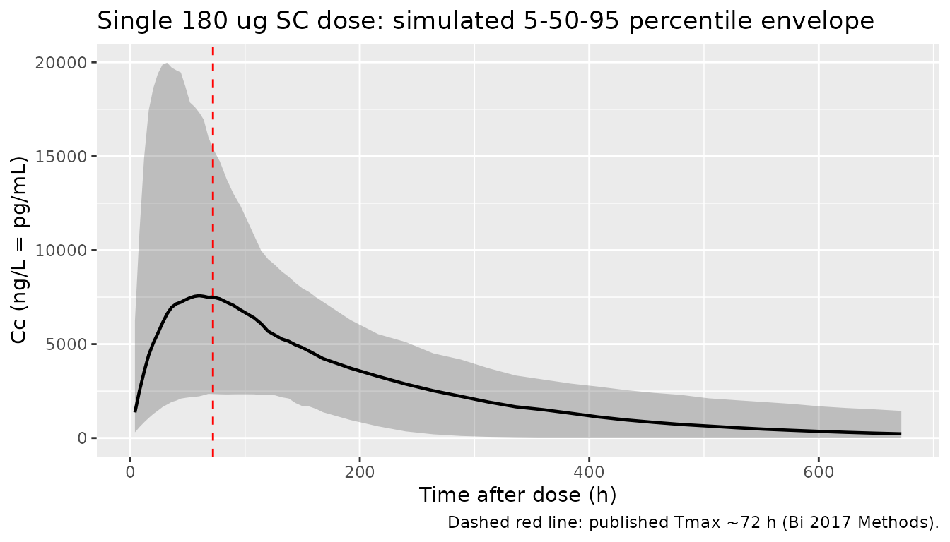
Typical-value Tmax sanity check
For a single dose with first-order absorption and first-order
elimination, the typical-value Tmax is
log(ka/kel) / (ka - kel). Using the Table 2 point estimates
and a typical subject (CRCL = 91.39 mL/min, BMI = 23.41 kg/m^2):
ka  <- 0.028
cl  <- 0.094
v   <- 15.6
kel <- cl / v
tmax_pred <- log(ka / kel) / (ka - kel)
round(tmax_pred, 1)
#> [1] 69.9
The closed-form Tmax matches the ~72 h value reported by Bi 2017.
Covariate-effect direction
Bi 2017 Discussion summarises the covariate directions: clearance increases with creatinine clearance (positive exponent 0.31), and volume of distribution increases with body mass index (positive exponent 1.81). The simulation below holds one covariate at its cohort mean while varying the other across the observed range; the plots show the typical-value (zero IIV) Cc trajectory.
mod_typical <- mod |> rxode2::zeroRe()

sweep_cov <- function(crcl, bmi) {
  ev_one <- tibble::tibble(id = 1L, time = 0, amt = dose_ng,
                            cmt = "depot", evid = 1L,
                            BMI = bmi, CRCL = crcl)
  ev_obs <- tibble::tibble(id = 1L, time = obs_times,
                            amt = 0, cmt = NA_character_, evid = 0L,
                            BMI = bmi, CRCL = crcl)
  ev <- dplyr::bind_rows(ev_one, ev_obs) |>
    dplyr::arrange(time, dplyr::desc(evid))
  rxode2::rxSolve(mod_typical, events = ev, keep = c("BMI", "CRCL")) |>
    as.data.frame() |>
    tibble::as_tibble() |>
    dplyr::mutate(CRCL = crcl, BMI = bmi)
}

crcl_levels <- c(45, 90, 150)     # spans Bi 2017 Table 1 range
bmi_levels  <- c(18, 23.41, 30)   # below mean, mean, above mean

# Vary CRCL at BMI = 23.41
sweep_crcl <- dplyr::bind_rows(lapply(crcl_levels, function(x) sweep_cov(x, 23.41)))
#> ℹ omega/sigma items treated as zero: 'etalcl', 'etalvc', 'etalka'
#> ℹ omega/sigma items treated as zero: 'etalcl', 'etalvc', 'etalka'
#> ℹ omega/sigma items treated as zero: 'etalcl', 'etalvc', 'etalka'
# Vary BMI at CRCL = 91.39
sweep_bmi  <- dplyr::bind_rows(lapply(bmi_levels,  function(x) sweep_cov(91.39, x)))
#> ℹ omega/sigma items treated as zero: 'etalcl', 'etalvc', 'etalka'
#> ℹ omega/sigma items treated as zero: 'etalcl', 'etalvc', 'etalka'
#> ℹ omega/sigma items treated as zero: 'etalcl', 'etalvc', 'etalka'

p_crcl <- sweep_crcl |>
  dplyr::filter(!is.na(Cc), time > 0) |>
  ggplot(aes(time, Cc, colour = factor(CRCL))) +
  geom_line(linewidth = 0.8) +
  labs(x = "Time (h)", y = "Cc (ng/L)",
       colour = "CRCL (mL/min)",
       title = "CRCL effect on CL (BMI = 23.41)") +
  theme(legend.position = "bottom")

p_bmi <- sweep_bmi |>
  dplyr::filter(!is.na(Cc), time > 0) |>
  ggplot(aes(time, Cc, colour = factor(BMI))) +
  geom_line(linewidth = 0.8) +
  labs(x = "Time (h)", y = "Cc (ng/L)",
       colour = "BMI (kg/m^2)",
       title = "BMI effect on V (CRCL = 91.39)") +
  theme(legend.position = "bottom")

print(p_crcl)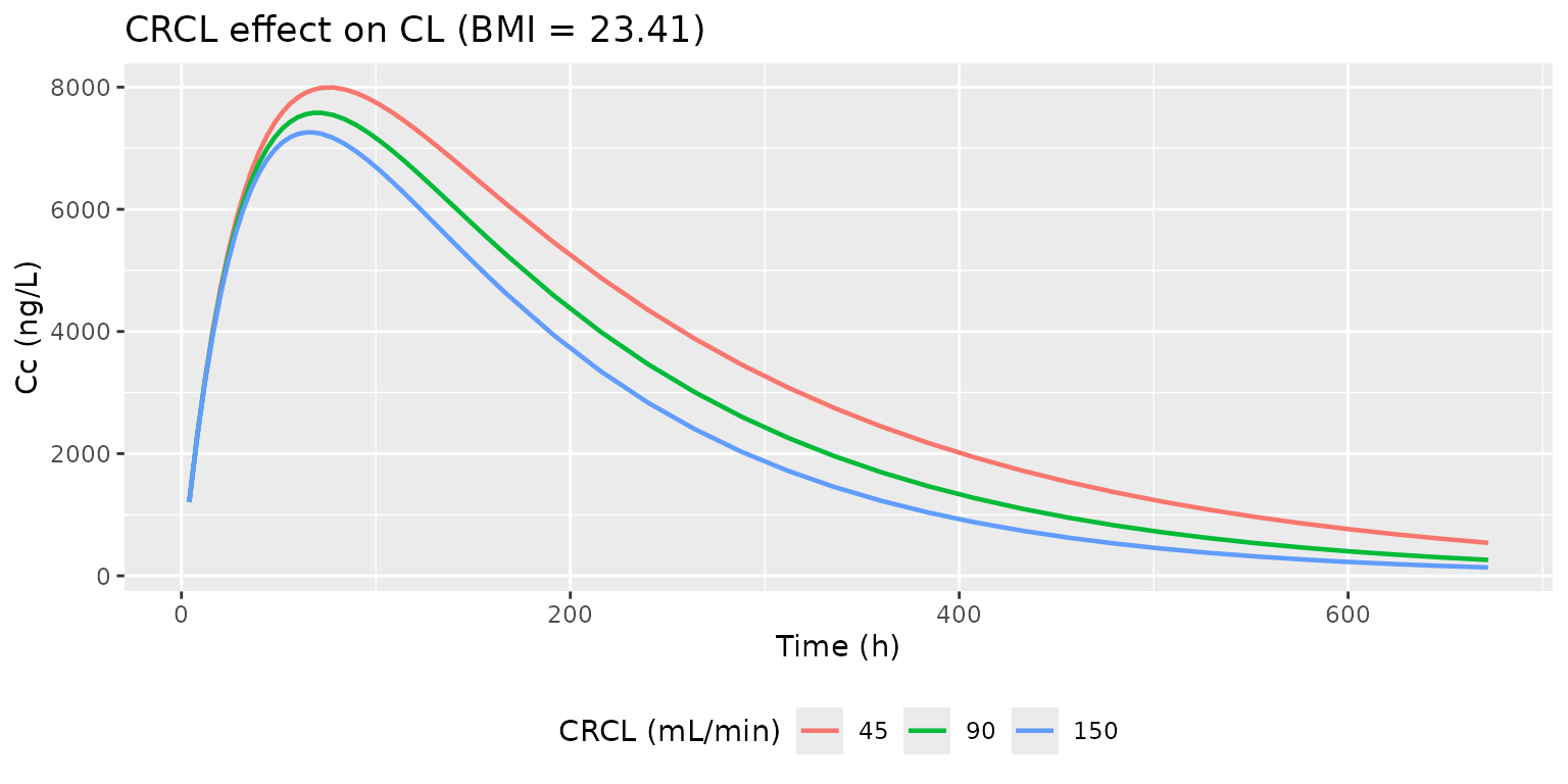
print(p_bmi)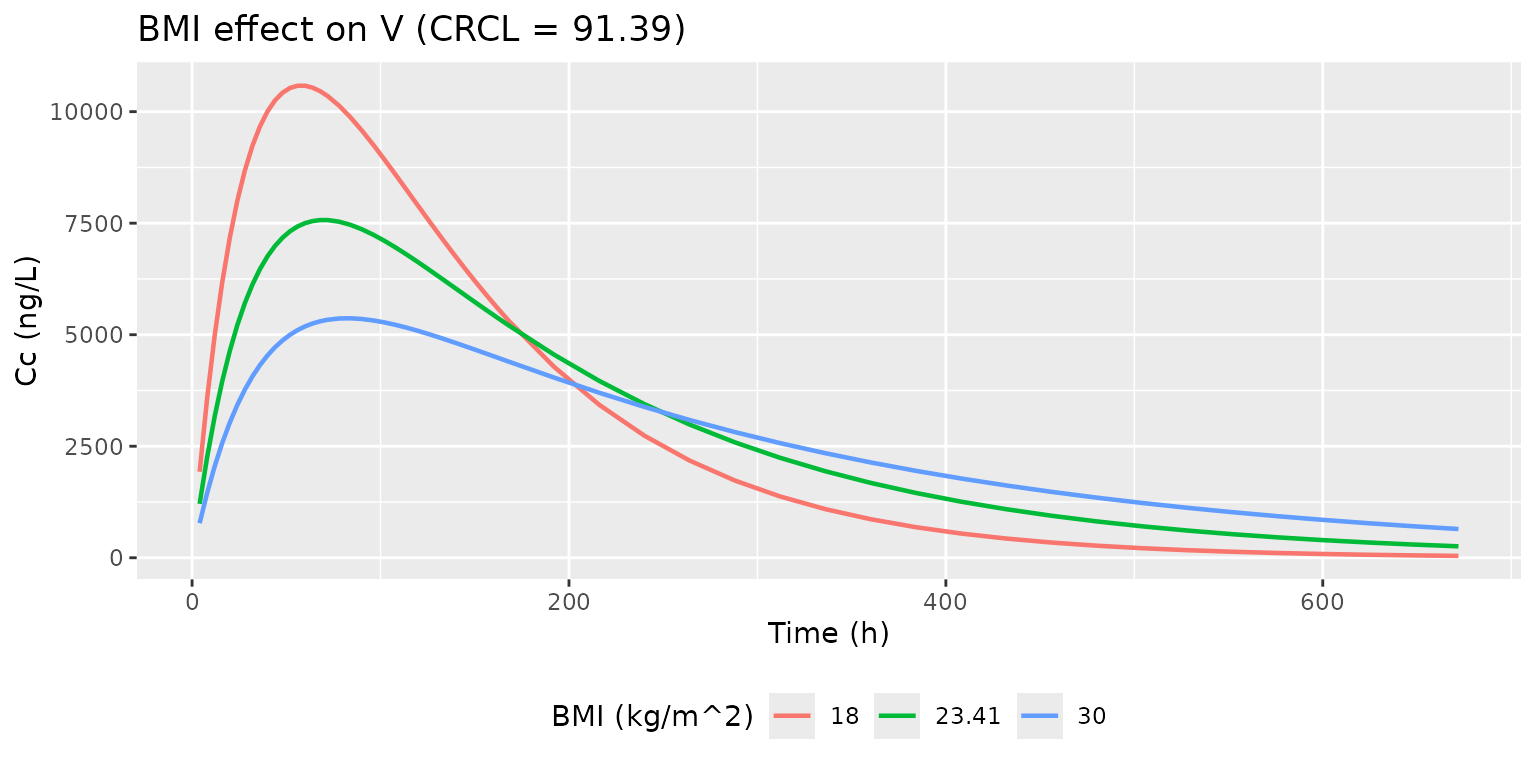
PKNCA validation
PKNCA gives Cmax, Tmax, AUC0-inf and terminal half-life for the
simulated cohort. Because Bi 2017 enrolled a single dose level (180 ug
SC weekly) and did not stratify by treatment, all subjects share one
grouping level (treatment = "180 ug SC") so the formula’s
left-hand grouping is structural rather than comparative.
sim_nca <- sim |>
  dplyr::filter(!is.na(Cc)) |>
  dplyr::mutate(treatment = "180 ug SC") |>
  dplyr::select(id, time, Cc, treatment)

dose_df <- doses |>
  dplyr::mutate(treatment = "180 ug SC") |>
  dplyr::select(id, time, amt, treatment)

conc_obj <- PKNCA::PKNCAconc(sim_nca, Cc ~ time | treatment + id,
                             concu = "ng/L", timeu = "hour")
dose_obj <- PKNCA::PKNCAdose(dose_df, amt ~ time | treatment + id,
                             doseu = "ng")

intervals <- data.frame(
  start       = 0,
  end         = Inf,
  cmax        = TRUE,
  tmax        = TRUE,
  aucinf.obs  = TRUE,
  half.life   = TRUE
)

nca_res <- PKNCA::pk.nca(PKNCA::PKNCAdata(conc_obj, dose_obj,
                                          intervals = intervals))

nca_tbl <- as.data.frame(nca_res$result) |>
  dplyr::filter(PPTESTCD %in% c("cmax", "tmax", "aucinf.obs", "half.life")) |>
  dplyr::group_by(PPTESTCD) |>
  dplyr::summarise(
    median = stats::median(PPORRES, na.rm = TRUE),
    q05    = stats::quantile(PPORRES, 0.05, na.rm = TRUE),
    q95    = stats::quantile(PPORRES, 0.95, na.rm = TRUE),
    .groups = "drop"
  )

knitr::kable(nca_tbl,
             digits = 2,
caption = "Simulated single-dose NCA for 180 ug SC peginterferon alfa-2a; median and 5-95th percentile across the virtual cohort.")| PPTESTCD | median | q05 | q95 |
|---|---|---|---|
| aucinf.obs | 1940619.20 | 1146685.98 | 3105318.80 |
| cmax | 7758.77 | 2368.66 | 19986.38 |
| half.life | 111.71 | 30.78 | 516.99 |
| tmax | 64.00 | 31.80 | 138.30 |
Comparison against published values
Bi 2017 does not tabulate per-subject NCA from their own data set, so the direct paper-vs-simulation table at this dose level is limited. The publication cites an earlier study (reference 7) that reported between-subject CV for AUC0-t = 36.0%, t1/2Z = 33.7%, Tmax = 30.2%, Cmax = 36.6% in a preliminary peginterferon alfa-2a PK study; the spreads in the table above are broadly consistent with those magnitudes. The simulated typical Tmax (~72 h) matches Bi 2017’s reported Tmax exactly.
Assumptions and deviations
- Bioavailability is held at F = 1 because Bi 2017 only had SC data (no IV reference); the published CL and V are therefore apparent (CL/F, V/F). Doses are entered in ng to keep the unit chain (ng / L) -> (ng/L) clean.
- Concentration units. Bi 2017 reports the additive residual SD as 0.32 ng/L (Table 2 footnote on units). 1 ng/L = 1 pg/mL; the assay LLOQ was 15 pg/mL = 15 ng/L (Pestka Biomedical Laboratories Human IFN-alpha ELISA). The vignette plots and PKNCA work in ng/L throughout.
-
IIV variance encoding. Bi 2017 Table 2 reports IIV
as percent CV. The internal variance entries in
ini()use the log-normal conversionomega^2 = log(CV^2 + 1). For the highest CV (V at 101%) this differs materially from the naiveomega = CVshortcut (0.703 vs 1.020); the conversion is documented in the model file. - Covariate independence in the virtual cohort. Bi 2017 Figure 1 documents non-zero correlations among CRCL, age, weight, and BMI in the observed cohort. The vignette samples BMI and CRCL independently because the structural model only depends on the joint distribution through marginal effects; the typical-value sensitivity check conditions on covariate values directly to make the direction of each effect visible.
-
Race / ethnicity. Bi 2017 does not tabulate race;
the cohort is Chinese (single-center, Beijing).
population$race_ethnicitycaptures this; the structural model has no race covariate so the virtual cohort does not need a race column. - Dosing convention. Doses in the source data set spanned 50000-180000 ng (50-180 ug) per Table 1; the vignette simulates the standard 180 ug weekly regimen described in the Introduction. The model is linear in dose, so the Cmax and AUC values scale proportionally with the prescribed dose.
-
No flip-flop guard. The IIV on V (101% CV) and Ka
(64% CV) is large enough that a small fraction of simulated individuals
can have
ka < kel. This matches the published parameter estimates and is not guarded in the model file; if a user needs strict first-order absorption, truncate the virtual cohort or sample IIV from a constrained joint distribution outside the model.