Allopurinol (Wright 2016)
Source:vignettes/articles/Wright_2016_allopurinol.Rmd
Wright_2016_allopurinol.RmdModel and source
- Citation: Wright DFB, Duffull SB, Merriman TR, Dalbeth N, Barclay ML, Stamp LK. Predicting allopurinol response in patients with gout. Br J Clin Pharmacol. 2016 Feb;81(2):277-289. doi:10.1111/bcp.12799
- Article: https://doi.org/10.1111/bcp.12799
The model is a one-compartment population PK-PD model for allopurinol (via the active metabolite oxypurinol) and plasma urate in adults with gout. Oxypurinol disposition is a one-compartment, first-order-absorption / first-order- elimination structure with Ka fixed at 1.09 1/h. Apparent oxypurinol clearance (CL/F_oxy) is allometrically scaled on fat-free mass and power-scaled on Cockcroft-Gault creatinine clearance standardised to 70 kg; when a thiazide or loop diuretic is coadministered, CL/F_oxy is reduced by 26%. Apparent oxypurinol volume (V/F_oxy) is allometrically scaled on total body weight (exponent fixed at 1.0) and shares its IIV with CL/F_oxy via a fixed fractional scaler (Bonate 2006 fractional-effect parameterisation; F_v_oxy = 0.0355).
Plasma urate is described by a direct-effect sigmoidal Emax inhibition of urate production on top of a baseline urate U0. The baseline is power-scaled on renal function (lower renal function -> mildly higher U0; exponent -0.119) and multiplicatively higher with concomitant diuretic (+14%). A turnover model for urate was tested by the authors but did not improve the fit and was unstable.
Population
The model was fit to the pooled five-study cohort summarised in Wright 2016 Table 2: 133 gout patients (87% male) from New Zealand. Median age 60 years (range 27 to 83), median total body weight 94 kg (range 51 to 171), median creatinine clearance 68 mL/min (range 12 to 125, raw Cockcroft-Gault). Roughly 20% of subjects were of Maori or Pacific Islander descent consistent with the high regional prevalence of severe gout. 33% (44 of 133) were on a thiazide or loop diuretic at study entry. The pooled dataset included 1105 oxypurinol and 1162 urate plasma concentrations across the five studies (Study 1 was the largest, n = 74, from Stamp 2011). Allopurinol daily doses ranged 50-700 mg (median 300 mg at study entry).
The same information is available programmatically via the model’s
population metadata:
pop <- readModelDb("Wright_2016_allopurinol")()$population
str(pop, max.level = 1, give.attr = FALSE)
#> List of 18
#>  $ species         : chr "human"
#>  $ n_subjects      : int 133
#>  $ n_studies       : int 5
#>  $ age_range       : chr "27 to 83 years"
#>  $ age_median      : chr "60 years"
#>  $ weight_range    : chr "51 to 171 kg total body weight"
#>  $ weight_median   : chr "94 kg total body weight"
#>  $ sex_female_pct  : num 12.7
#>  $ race_ethnicity  : chr "European 78.2%, Maori or Pacific Islander 20.3%, East Asian 0.8% (one Korean subject), South Asian 0.8% (one In"| __truncated__
#>  $ disease_state   : chr "Adults with gout; 29 patients were allopurinol-naive (initiating therapy) and 104 were on chronic allopurinol f"| __truncated__
#>  $ dose_range      : chr "Allopurinol 50-700 mg/day oral (median 300 mg/day at study entry; Wright 2016 Table 2 totals)."
#>  $ regions         : chr "New Zealand (multi-centre; Christchurch and Auckland)."
#>  $ crcl_range      : chr "12 to 125 mL/min total cohort range (median 68 mL/min ~= 4.08 L/h standardised to 70 kg; Wright 2016 Table 2)."
#>  $ co_medication   : chr "Concomitant medications tested as PD covariates and retained: thiazide or loop diuretic (33%). Tested without r"| __truncated__
#>  $ genotypes_tested: chr "Renal-urate-transporter SNPs rs11942223 (SLC2A9), rs2231142 (ABCG2), rs1183201 (NPT1/SLC17A1), and rs3825018 (U"| __truncated__
#>  $ samples         : chr "1105 oxypurinol and 1162 urate plasma concentrations from 133 gout patients (Wright 2016 Results). Concentratio"| __truncated__
#>  $ studies_notes   : chr "Five-study pooled analysis: Study 1 (n=74; Stamp 2011 [19], the largest single cohort), Study 2 (n=10; Stamp 20"| __truncated__
#>  $ notes           : chr "Allopurinol (parent) is NOT modelled because (a) the allopurinol-parent model was found to be unstable in prior"| __truncated__
Source trace
The per-parameter origin is recorded as an in-file comment next to
each ini() entry in
inst/modeldb/specificDrugs/Wright_2016_allopurinol.R. The
table below collects them in one place for review.
| Equation / parameter | Value | Source location |
|---|---|---|
lka = log(1.09) (fixed) |
Ka = 1.09 1/h | Wright 2016 Table 3 (Ka fixed both base and final columns) |
lcl = log(1.32) |
CL/F_oxy = 1.32 L/h at reference | Wright 2016 Table 3 thetaCL (RSE 3.9%) |
lvc = log(41.6) |
V/F_oxy = 41.6 L at reference TBW | Wright 2016 Table 3 thetaV (RSE 3.0%) |
e_ffm_cl = 0.75 (fixed) |
FFM allometric exponent on CL | Wright 2016 Methods (Anderson and Holford) |
e_wt_vc = 1.0 (fixed) |
TBW allometric exponent on V | Wright 2016 Methods (Anderson and Holford) |
e_crcl_cl = 0.587 |
thetaRFexp | Wright 2016 Table 3 (RSE 11.7%) |
e_conmed_diuretic_cl = 0.740 |
thetadiuretic | Wright 2016 Table 3 (RSE 6.4%) |
lemax = log(0.409) |
Emax = 0.409 | Wright 2016 Table 3 Emax (RSE 12%) |
lec50 = log(83.9) |
C50 = 83.9 umol/L | Wright 2016 Table 3 C50 (RSE 17.4%) |
lhill = log(1.30) |
lambda (Hill) = 1.30 | Wright 2016 Table 3 lambda (RSE 11%) |
lrbase = log(0.511) |
U0 = 0.511 mmol/L | Wright 2016 Table 3 U0 (RSE 2.3%) |
e_crcl_rbase = -0.119 |
thetaE0_RFexp | Wright 2016 Table 3 (RSE 21.6%) |
e_conmed_diuretic_rbase = 1.14 |
thetaE0_diuretic | Wright 2016 Table 3 (RSE 1.8%) |
etalcl ~ 0.0586 |
omega_CL = 24.2% | Wright 2016 Table 3 omegaCL (RSE 15.5%) |
F_v_oxy = 0.0355 (fixed) |
V fractional shared-eta scaler | Wright 2016 Table 3 F_omegaV_oxy |
etalka ~ fixed(0.347) |
omega_Ka = 58.9% fixed | Wright 2016 Table 3 (fixed both columns) |
(etalrbase, etalemax, etalec50) block |
omega_U0 14.2%, omega_Emax 35.9%, omega_C50 60.7%; Cov(emax, U0) = 0.025; Cov(emax, C50) = 0.193; Cov(U0, C50) = 0.011 | Wright 2016 Table 3 omega and Covar rows |
propSd = 0.199 |
Cc proportional residual 19.9% CV | Wright 2016 Table 3 oxypurinol sigma_prop |
addSd = fixed(0.001) |
Cc additive residual (fixed, negligible) | Wright 2016 Table 3 footer |
addSd_Eurate = 0.037 |
Urate additive residual 0.037 mmol/L (Study 1 / 3 representative) | Wright 2016 Table 3 Study 1 sigma_add |
propSd_Eurate = fixed(0.001) |
Urate proportional residual (fixed, negligible) | Wright 2016 Table 3 footer |
ODE: d/dt(depot) = -ka * depot
|
n/a | Wright 2016 PK Models section |
ODE: d/dt(central) = ka * depot - kel * central
|
n/a | Wright 2016 PK Models section |
Observable: Cc = central / vc * 1000 / MW_allop
(MW_allop = 136.11 g/mol) |
n/a | Implicit molar conversion: dose mg allopurinol -> umol/L oxypurinol |
Observable:
Eurate = U0 * (1 - Emax * Cc^lambda / (C50^lambda + Cc^lambda))
|
n/a | Wright 2016 Results equation set (page 282) |
Virtual cohort
Original observed data are not publicly available. The figures below use virtual populations whose covariate distributions approximate the published trial demographics: a male-majority adult-gout cohort with median total body weight 94 kg and median CRCL standardised to 70 kg ~= 4.08 L/h (= 68 mL/min in the raw Cockcroft-Gault expression).
Cohort size is kept at the package’s cap of 200 subjects per arm (adequate for VPC; larger cohorts increase render time without validation benefit).
set.seed(20260630)

# Janmahasatian fat-free mass (kg) from total body weight (kg), height
# (cm), and SEXF (1 = female, 0 = male). Wright 2016 cites this formula
# as the FFM derivation used in the model fit.
ffm_janmahasatian <- function(WT, HT_cm, SEXF) {
  HT_m  <- HT_cm / 100
  BMI   <- WT / HT_m^2
  WHS_max <- ifelse(SEXF == 1, 37.99, 42.92)
  WHS_50  <- ifelse(SEXF == 1, 35.98, 30.93)
  WHS_max * HT_m^2 * (WT / (WHS_50 * HT_m^2 + WT))
}

# Build one cohort of n synthetic subjects. id_offset shifts the integer
# id range so cohorts can be bind_rows()-ed without colliding.
make_cohort <- function(n, daily_dose_mg, diuretic = 0L, id_offset = 0L,
                        cohort_label = "") {
  tibble::tibble(
    id     = id_offset + seq_len(n),
    SEXF   = rbinom(n, 1, prob = 0.13),                       # ~13% female per Wright 2016 Table 2
    WT     = pmin(pmax(round(rnorm(n, mean = 94, sd = 18)), 51), 171),
    HT_cm  = pmin(pmax(round(rnorm(n, mean = 173, sd = 9)), 150), 195),
    CRCL_mLmin = pmin(pmax(round(rnorm(n, mean = 68, sd = 22)), 20), 125),
    CONMED_DIURETIC = as.integer(diuretic),
    cohort   = cohort_label,
    treatment = paste0(daily_dose_mg, " mg/day"),
    daily_dose_mg = daily_dose_mg
  ) |>
    dplyr::mutate(
      FFM  = ffm_janmahasatian(WT, HT_cm, SEXF),
      # Wright 2016's CRCL is Cockcroft-Gault expressed in L/h
      # standardised to 70 kg: CRCL_L_h_70kg = CRCL_mLmin * (70 / WT) / 16.6667
      # 16.6667 mL/min per L/h conversion.
      CRCL = CRCL_mLmin * (70 / WT) / 16.6667
    )
}

# Build a dosing + observation event table for one cohort. The dose is
# allopurinol mg given q24h for `dose_days` consecutive days, with urate
# and oxypurinol sampling at one-hour intervals over the final
# 24-hour interval (= steady-state-relevant window) and a baseline
# pre-dose sample at t = 0.
build_events <- function(subj, dose_days = 28, obs_grid_h = NULL) {
  if (is.null(obs_grid_h)) {
    # observation grid: every 4 hours over the LAST 24 h plus a baseline
    last_day_start <- (dose_days - 1) * 24
    obs_grid_h <- c(0, seq(last_day_start, last_day_start + 24, by = 4))
  }
  doses <- subj |>
    dplyr::select(id, daily_dose_mg, FFM, WT, CRCL, CONMED_DIURETIC,
                  cohort, treatment) |>
    tidyr::expand_grid(time = seq(0, by = 24, length.out = dose_days)) |>
    dplyr::mutate(amt = daily_dose_mg, evid = 1L, cmt = "depot",
                  dvid = NA_integer_)
  obs_cc <- subj |>
    dplyr::select(id, FFM, WT, CRCL, CONMED_DIURETIC, cohort, treatment) |>
    tidyr::expand_grid(time = obs_grid_h) |>
    dplyr::mutate(amt = NA_real_, evid = 0L, cmt = "Cc",
                  dvid = 1L)
  obs_urate <- subj |>
    dplyr::select(id, FFM, WT, CRCL, CONMED_DIURETIC, cohort, treatment) |>
    tidyr::expand_grid(time = obs_grid_h) |>
    dplyr::mutate(amt = NA_real_, evid = 0L, cmt = "Eurate",
                  dvid = 2L)
  dplyr::bind_rows(doses, obs_cc, obs_urate) |>
    dplyr::arrange(id, time, evid)
}
# Six dose levels at fixed adult-typical covariates; reproduces the
# Wright 2016 Figure 3 stratification (100 / 200 / 300 / 400 / 600 mg
# daily for ~3 months). Wright 2016 uses 1000 subjects per dose for
# its Figure 3 simulation; we use the package's 200/arm cohort cap.
N_PER_ARM <- 200L
doses <- c(100, 200, 300, 400, 600)

cohorts <- dplyr::bind_rows(lapply(seq_along(doses), function(i) {
  make_cohort(n = N_PER_ARM,
              daily_dose_mg = doses[i],
              diuretic = 0L,
              id_offset = (i - 1L) * N_PER_ARM,
              cohort_label = paste0(doses[i], " mg/day"))
}))

events_dose <- build_events(cohorts, dose_days = 90)

# Assertion: ids disjoint and (id, time, evid) unique.
stopifnot(!anyDuplicated(unique(events_dose[, c("id", "time", "evid")])))
Simulation
mod <- readModelDb("Wright_2016_allopurinol")
sim <- rxode2::rxSolve(mod, events = events_dose,
                       keep = c("cohort", "treatment", "WT",
                                "CRCL", "CONMED_DIURETIC")) |>
  as.data.frame()
#> ℹ parameter labels from comments will be replaced by 'label()'
nrow(sim)
#> [1] 16000
Replicate Figure 3 – percent urate reduction by daily dose
Wright 2016 Figure 3 compares the model-predicted distribution of percent urate reduction (from baseline) under 100, 200, 300, 400, and 600 mg daily allopurinol against external literature data. We reproduce the model side of that figure by computing the percent reduction from baseline (= U0 at the typical patient covariates) at steady state.
# Steady-state percent reduction from baseline urate, per subject:
# pick the urate observation at the last simulated time point in each
# subject's series (= near-steady-state under chronic q24h dosing).
ss <- sim |>
  dplyr::filter(!is.na(Eurate)) |>
  dplyr::group_by(id, cohort, treatment) |>
  dplyr::filter(time == max(time)) |>
  dplyr::ungroup()

# Baseline U0 per subject = Eurate at t = 0 (pre-dose).
baseline <- sim |>
  dplyr::filter(time == 0, !is.na(Eurate)) |>
  dplyr::select(id, baseline = Eurate)

ss <- ss |>
  dplyr::inner_join(baseline, by = "id") |>
  dplyr::mutate(pct_reduction = 100 * (baseline - Eurate) / baseline,
                treatment = factor(treatment, levels = paste0(doses, " mg/day")))
#> Warning in dplyr::inner_join(ss, baseline, by = "id"): Detected an unexpected many-to-many relationship between `x` and `y`.
#> ℹ Row 1 of `x` matches multiple rows in `y`.
#> ℹ Row 1 of `y` matches multiple rows in `x`.
#> ℹ If a many-to-many relationship is expected, set `relationship =
#>   "many-to-many"` to silence this warning.

ggplot(ss, aes(treatment, pct_reduction)) +
  geom_boxplot(fill = "grey80") +
  labs(x = "Allopurinol daily dose",
       y = "% reduction in plasma urate from baseline",
       title = "Replicates the model side of Figure 3 (Wright 2016)",
       caption = "Each box = 200 simulated subjects at the typical adult-gout covariate distribution.") +
  theme_minimal(base_size = 11) +
  theme(axis.text.x = element_text(angle = 30, hjust = 1))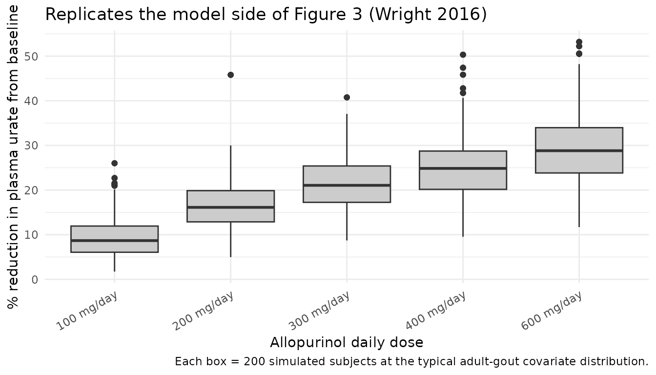
# Median per dose (for the comparison table below).
median_table <- ss |>
  dplyr::group_by(treatment) |>
  dplyr::summarise(median_pct = round(median(pct_reduction), 1),
                   q25_pct    = round(quantile(pct_reduction, 0.25), 1),
                   q75_pct    = round(quantile(pct_reduction, 0.75), 1),
                   .groups = "drop")

median_table |>
  dplyr::rename("Treatment"                = treatment,
                "Median % reduction"       = median_pct,
                "Q1 % reduction"           = q25_pct,
                "Q3 % reduction"           = q75_pct) |>
knitr::kable(caption = "Simulated steady-state percent urate reduction by daily allopurinol dose, typical-cohort covariates.")| Treatment | Median % reduction | Q1 % reduction | Q3 % reduction |
|---|---|---|---|
| 100 mg/day | 8.7 | 6.1 | 11.9 |
| 200 mg/day | 16.1 | 12.9 | 19.9 |
| 300 mg/day | 21.1 | 17.3 | 25.4 |
| 400 mg/day | 24.9 | 20.2 | 28.7 |
| 600 mg/day | 28.8 | 23.8 | 34.0 |
Replicate dosing predictions – Table 4 (no diuretic, CLcr 50-70)
Wright 2016 Table 4 lists the maintenance dose required to achieve plasma urate <= 0.36 mmol/L in > 75% of subjects across a grid of body weights and CRCL strata. Here we reproduce the > 75% success criterion for the CLcr 50-70 mL/min stratum at 70 kg total body weight, no diuretic (Table 4 target: 350 mg/day).
# Build a 70 kg adult, no-diuretic cohort with CRCL drawn from a
# uniform U(50, 70) mL/min, then test three candidate doses around
# the Table 4 target of 350 mg/day.
make_table4_cohort <- function(n, daily_dose_mg, id_offset, cohort_label) {
  tibble::tibble(
    id = id_offset + seq_len(n),
    SEXF = 0L,
    WT = 70,
    HT_cm = 175,
    CRCL_mLmin = runif(n, 50, 70),
    CONMED_DIURETIC = 0L,
    cohort = cohort_label,
    treatment = paste0(daily_dose_mg, " mg/day"),
    daily_dose_mg = daily_dose_mg
  ) |>
    dplyr::mutate(
      FFM = ffm_janmahasatian(WT, HT_cm, SEXF),
      CRCL = CRCL_mLmin * (70 / WT) / 16.6667
    )
}

t4_cohorts <- dplyr::bind_rows(
  make_table4_cohort(N_PER_ARM, 300L, id_offset = 0L,             cohort_label = "300 mg/day"),
  make_table4_cohort(N_PER_ARM, 350L, id_offset = N_PER_ARM,      cohort_label = "350 mg/day"),
  make_table4_cohort(N_PER_ARM, 400L, id_offset = 2L * N_PER_ARM, cohort_label = "400 mg/day")
)
ev_t4 <- build_events(t4_cohorts, dose_days = 90)
stopifnot(!anyDuplicated(unique(ev_t4[, c("id", "time", "evid")])))

sim_t4 <- rxode2::rxSolve(mod, events = ev_t4,
                          keep = c("cohort", "treatment", "WT", "CRCL")) |>
  as.data.frame()

# Steady-state urate at the last sampled time.
ss_t4 <- sim_t4 |>
  dplyr::filter(!is.na(Eurate)) |>
  dplyr::group_by(id, treatment) |>
  dplyr::filter(time == max(time)) |>
  dplyr::ungroup() |>
  dplyr::mutate(below_target = Eurate <= 0.36)

success_table <- ss_t4 |>
  dplyr::group_by(treatment) |>
  dplyr::summarise(pct_below_target = round(100 * mean(below_target), 1),
                   median_urate = round(median(Eurate), 3),
                   .groups = "drop")

success_table |>
  dplyr::rename("Treatment" = treatment,
                "% subjects with urate <= 0.36 mmol/L" = pct_below_target,
                "Median steady-state urate (mmol/L)" = median_urate) |>
knitr::kable(caption = "Replicate of Wright 2016 Table 4 row: 70 kg, no diuretic, CLcr 50-70 mL/min. Table 4 target dose = 350 mg/day.")| Treatment | % subjects with urate <= 0.36 mmol/L | Median steady-state urate (mmol/L) |
|---|---|---|
| 300 mg/day | 5.0 | 0.440 |
| 350 mg/day | 6.5 | 0.421 |
| 400 mg/day | 13.5 | 0.400 |
PKNCA validation on oxypurinol
Use PKNCA to compute Cmax, Tmax, and AUC over a 24-hour steady-state interval for the 300 mg/day dose group (the typical clinical regimen). Wright 2016 does not publish formal NCA for oxypurinol (only descriptive medians per study, Table 2), so this section is a sanity check that the PK structure produces plausible numbers rather than a head-to-head comparison.
sim_for_nca <- sim |>
  dplyr::filter(treatment == "300 mg/day", !is.na(Cc))

# Carve out the last 24 h of the simulation as a steady-state interval.
ss_window_start <- max(sim_for_nca$time) - 24

sim_nca <- sim_for_nca |>
  dplyr::filter(time >= ss_window_start) |>
  dplyr::mutate(time = time - ss_window_start) |>
  dplyr::select(id, time, Cc, treatment)

# Guarantee a time=0 (relative to interval start) Cc value per (id, treatment).
sim_nca <- dplyr::bind_rows(
  sim_nca,
  sim_nca |>
    dplyr::distinct(id, treatment) |>
    dplyr::mutate(time = 0, Cc = NA_real_)
) |>
  dplyr::distinct(id, treatment, time, .keep_all = TRUE) |>
  dplyr::arrange(id, treatment, time) |>
  tidyr::fill(Cc, .direction = "downup") |>
  dplyr::filter(!is.na(Cc))

conc_obj <- PKNCA::PKNCAconc(sim_nca, Cc ~ time | treatment + id)

dose_df <- events_dose |>
  dplyr::filter(evid == 1, treatment == "300 mg/day") |>
  dplyr::group_by(id) |>
  dplyr::filter(time == max(time)) |>
  dplyr::ungroup() |>
  dplyr::mutate(time = 0) |>
  dplyr::select(id, time, amt, treatment)

dose_obj <- PKNCA::PKNCAdose(dose_df, amt ~ time | treatment + id)

intervals <- data.frame(
  start = 0, end = 24, cmax = TRUE, tmax = TRUE, auclast = TRUE
)
nca_data <- PKNCA::PKNCAdata(conc_obj, dose_obj, intervals = intervals)
nca_res <- PKNCA::pk.nca(nca_data)

nca_summary <- as.data.frame(nca_res$result) |>
  dplyr::filter(PPTESTCD %in% c("cmax", "tmax", "auclast")) |>
  dplyr::group_by(treatment, PPTESTCD) |>
  dplyr::summarise(median = round(median(PPORRES, na.rm = TRUE), 2),
                   .groups = "drop") |>
  tidyr::pivot_wider(names_from = PPTESTCD, values_from = median)

nca_summary |>
  dplyr::rename("Treatment"   = treatment,
                "Median Cmax (umol/L)" = cmax,
                "Median Tmax (h)"      = tmax,
                "Median AUC0-24 (umol*h/L)" = auclast) |>
knitr::kable(caption = "Simulated oxypurinol steady-state NCA (300 mg/day, no diuretic, 200 subjects). Wright 2016 reports a typical patient's average oxypurinol concentration of ~70 umol/L at 226 mg/day (Discussion); the 300 mg/day arm here should sit slightly above that value.")| Treatment | Median AUC0-24 (umol*h/L) | Median Cmax (umol/L) | Median Tmax (h) |
|---|---|---|---|
| 300 mg/day | 2757.27 | 130.61 | 4 |
Assumptions and deviations
- Year on the citation. The paper is sometimes cited as “Wright 2015” because the publisher posted the accepted-article PDF online on 9 October 2015. The final, citeable BJCP volume issue (81:2, 277-289) is dated February 2016 with the same DOI (10.1111/bcp.12799); we use the 2016 year throughout the model file, vignette, and filename for the canonical citation, matching how the paper is indexed in PubMed.
-
Per-study urate residual error. Wright 2016 reports
five different urate additive residual SDs across the five pooled
studies (0.021, 0.022, 0.037, 0.037, 0.054 mmol/L). The model file
retains a single representative value of 0.037 mmol/L (Studies 1 and 3;
Study 1 is the largest single sub-cohort at n = 74 of 133 and the median
across studies). A user wanting to reproduce a specific sub-study’s VPC
should override
addSd_Eurateaccordingly. -
CONMED_DIURETIC class membership. Wright 2016’s
CONMED_DIURETIC captures thiazide diuretics OR loop diuretics (per
Wright 2016 Table 4 footer). This is NARROWER than the Stocker 2012
oxypurinol precedent (
Stocker_2012_oxypurinol.R), which pools thiazide + loop + spironolactone into the same column. The two papers use the same canonical CONMED_DIURETIC column name; users simulating across both models must populate the indicator according to each paper’s own definition. - IIV scale convention. Wright 2016 reports omega values as “(CV%)” but the reported PD covariance block is only positive-definite when the reported %CV is interpreted as the log-scale SD directly (i.e., omega^2 = (CV / 100)^2) rather than the back-transformed CV (which would give omega^2 = log(1 + CV^2)). The model file uses the log-scale-SD interpretation throughout for internal consistency.
- V’s “fractional effect” IIV. Wright 2016 notes that BSV on V was not identifiable; only a single random effect was estimated for both CL and V, with V’s individual deviation a fixed fraction (F_v_oxy = 0.0355) of CL’s. We encode this exactly: V_i = V_pop exp(F_v_oxy etalcl), shared etalcl, with F_v_oxy held fixed.
- Dose unit and molar conversion. The dose entered into the model is allopurinol mass in mg. The model’s apparent CL/F_oxy and V/F_oxy absorb the implicit F_oxy (fraction absorbed * fraction metabolised to oxypurinol; 1:1 molar) so the central compartment carries allopurinol-equivalent mg. The observable Cc converts to umol/L oxypurinol using the allopurinol molecular weight 136.11 g/mol; this matches the paper’s apparent-CL definition and reproduces the cohort median oxypurinol concentration of ~70 umol/L at 226 mg/day reported in the Wright 2016 Discussion.
-
CRCL standardisation. The model expects CRCL in L/h
standardised to 70 kg (Wright 2016 reference: 100 mL/min/70 kg = 6
L/h/70 kg). The virtual cohort code in this vignette converts raw
Cockcroft-Gault mL/min to the 70-kg-standardised L/h form via
CRCL = CRCL_mLmin * (70 / WT) / 16.6667. Users supplying CRCL directly should standardise externally. -
Genotype covariates. Wright 2016 tested four
urate-transporter SNPs (SLC2A9, ABCG2, NPT1, URAT1) and one of them
(ABCG2 T-allele homozygote) approached significance on C50 (+40%) but
did not meet the backward-elimination criterion. The model file does not
include this effect because it was not retained; users who want to
explore it can add a multiplier on
lec50manually. - No external NCA validation. Wright 2016 does not publish formal NCA parameters for oxypurinol (only cohort medians; Table 2). The PKNCA block above is a sanity check, not a head-to-head comparison.