Aztreonam-avibactam (Xie 2025)

Model and source

• Citation: Xie R, Rogers H, Chow JW, Soto E, Raber SR. Population pharmacokinetic/pharmacodynamic modeling to optimize aztreonam-avibactam dose regimens for adult patients. Antimicrob Agents Chemother. 2025;69(8):e01950-24. doi:10.1128/aac.01950-24. All fixed-effect, random-effect and residual-error estimates are the ‘Final model (run 46)’ column of supplementary Table S3. The functional FORMS of the covariate relationships are not printed in Xie 2025; they are taken from the immediate structural predecessor by the same group, Das S, Riccobene T, Carrothers TJ, Wright JG, MacPherson M, Cristinacce A, McFadyen L, Xie R, Luckey A, Raber S. Dose selection for aztreonam-avibactam, including adjustments for renal impairment, for Phase IIa and Phase III evaluation. Eur J Clin Pharmacol. 2024;80(4):529-543. doi:10.1007/s00228-023-03609-x, supplementary Tables 4 and 5.

• Description: Simultaneous four-compartment (two compartments per drug) population PK model for the fixed-ratio (3:1) aztreonam-avibactam combination, fitted jointly to 4,914 aztreonam plasma samples from 431 subjects and 18,222 avibactam plasma samples from 2,635 subjects pooled across Phase 1, Phase 2a and Phase 3 aztreonam-avibactam studies plus the ceftazidime-avibactam development program (Xie 2025). Both drugs are given as zero-order intravenous infusions with first-order elimination. Body weight is an allometric covariate on CL, Vc, Q and Vp of both drugs with fixed exponents. Time-varying BSA-normalized creatinine clearance acts on the clearance of both drugs through a hinged relationship: a power function below 80 mL/min/1.73 m^2 and a linear function at or above it. Infection type shifts clearance and central volume, and avibactam additionally carries end-stage-renal-disease, hemodialysis, Chinese-race and APACHE II severity terms. The two drugs are linked by a four-way OMEGA block across aztreonam and avibactam CL and Vc, whose cross-drug correlations are 0.98 and 0.99. Aztreonam is the unsuffixed parent; avibactam carries the sibling-drug suffix _avi throughout.

• Article: https://doi.org/10.1128/aac.01950-24

• Supplement (Tables S1-S11, Figures S1-S6): available from the article landing page as aac.01950-24-s0001.docx

• Structural predecessor (covariate equation forms): https://doi.org/10.1007/s00228-023-03609-x

Aztreonam-avibactam is a fixed-ratio (3:1) monobactam / beta-lactamase-inhibitor combination approved in Europe in 2024 for complicated intra-abdominal infection (cIAI), complicated urinary tract infection (cUTI), hospital-acquired and ventilator-associated pneumonia, and other infections due to aerobic gram-negative organisms with limited treatment options. Xie 2025 added the two adult Phase 3 trials (REVISIT, ASSEMBLE) and two further Phase 1 studies to the previous data set and re-estimated a simultaneous population PK model for both analytes, then used it to confirm dose regimens across renal-function groups, to propose a simplified loading dose, and to derive a regimen for end-stage renal disease.

Both drugs are described by a two-compartment disposition model with zero-order infusion and first-order elimination, so the packaged model is a four-state system. What makes it a simultaneous model rather than two independent ones is the OMEGA block: aztreonam and avibactam clearance and central volume share a single 4x4 covariance block whose cross-drug correlations are 0.98 and 0.99 – “as expected for drugs that are both predominantly renally cleared”, in the paper’s words.

Population

The pooled analysis comprised 4,914 aztreonam plasma samples from 431 subjects and 18,222 avibactam plasma samples from 2,635 subjects. The avibactam data set is far larger because it carries the ceftazidime-avibactam development program in addition to the aztreonam-avibactam studies; this asymmetry is load-bearing for the covariate model, since cUTI is estimable for avibactam (707 subjects) but not for aztreonam (3 subjects), so several covariates are avibactam-only by necessity rather than by biology.

Subjects spanned 18-89 years and 28-190 kg, 38.6% female, and renal function from augmented renal clearance to end-stage renal disease. Baseline characteristics are in supplementary Tables S1 (aztreonam) and S2 (avibactam).

Population summary (model population metadata).

Field	Value
Species	human
Subjects	2,635
Concentrations	23,136
Age	18-89 years
Weight	28-190 kg
Female	38.6%
Disease states	healthy, cIAI, HAP/VAP, cUTI, bloodstream infection
Renal function	augmented renal clearance through end-stage renal disease

Source trace

Every ini() value is the “Final model (run 46)” column of supplementary Table S3. The covariate equation forms are not printed anywhere in Xie 2025, so they are taken from the immediate structural predecessor by the same author group, Das 2024 (supplementary Tables 4 and 5), which prints them verbatim.

Equation / parameter	Value	Source location
lcl, lvc, lq, lvp (aztreonam)	5.00 L/h, 7.01 L, 9.41 L/h, 6.12 L	Xie 2025 Table S3, theta1-theta4
lcl_avi, lvc_avi, lq_avi, lvp_avi	10.3 L/h, 12.6 L, 4.82 L/h, 6.95 L	Xie 2025 Table S3, theta5-theta8
lcl_dial_avi	17.9 L/h	Xie 2025 Table S3, theta12 (CL_AVI_DIAL)
e_wt_cl_q, e_wt_vc_vp	0.75, 1 (both fixed)	Xie 2025 Results, “allometric scaling with fixed exponents of 0.75 on CL and Q, and 1 on Vc and Vp”
e_crcl_cl_lt80, e_crcl_cl_ge80	0.502, 0.00383	Xie 2025 Table S3, theta9 / theta15
e_crcl_cl_lt80_avi, e_crcl_cl_ge80_avi	1.06, 0.00313	Xie 2025 Table S3, theta10 / theta16
form of the nCrCL hinge	(nCrCL/80)^p below 80; 1 + s*(nCrCL-80) at/above 80	Das 2024 Table S5, rows “theta7: CL, (CrCL/80)**theta7, CrCL <80” and “theta8: CL, (1+theta8*(CrCL-80)), CrCL >=80”
e_renalimp_esrd_cl_avi	-0.923	Xie 2025 Table S3, theta11
ESRD replaces rather than multiplies the nCrCL arm	n/a	Das 2024 Table S4, “theta8: CL, (nCrCL/80)**theta8, nCrCL <80 mL/min and not ESRD”
e_ciai_ph2_cl_avi, e_ciai_ph2_vc_avi	0.89, 1.64	Xie 2025 Table S3, theta13 / theta14 (Study2002)
e_cuti_vc_avi, e_cuti_cl_avi	1.5, 0.222	Xie 2025 Table S3, theta24 / theta26
e_ciai_habp_vabp_vc	0.931	Xie 2025 Table S3, theta25 (cIAI/NP on Vc); Results, “same cIAI and NP (HAP/VAP) effect on aztreonam and avibactam Vc”
e_ciai_cl_avi, e_ciai_cl	0.115, 0.279	Xie 2025 Table S3, theta27 / theta31
e_race_chinese_vc_avi	-0.145	Xie 2025 Table S3, theta29 (China on Vc_AVI)
e_apache_ii_sev_cl_avi	-0.118	Xie 2025 Table S3, theta30
proportional X*(1 + theta) form of the categorical effects	n/a	Das 2024 Table S5, e.g. “theta11: Population effect on Vc (cUTI), Vc*(1+theta11)”
4x4 OMEGA block (CL/Vc of both drugs)	40.2 / 60.8 / 43.5 / 65.2 %CV, six covariances	Xie 2025 Table S3, IIV and cov rows
Q-Vp avibactam OMEGA block	31.4 / 17.7 %CV, cov 0.0309	Xie 2025 Table S3; Results, “a covariance term between the avibactam IIVs in Q and Vp”
Residual error (4 aztreonam proportional strata, 1 avibactam)	12.5 / 22.4 / 40.3 / 53.3%, 20%	Xie 2025 Table S3, theta17-theta23
Unbound fractions used for the PK/PD targets	0.616 (ATM), 0.92 (AVI)	Xie 2025 Methods, “Predicted exposures for phase 3 trial patients”
Joint PK/PD target	60% fT>MIC 8 mg/L and 50% fT>CT 2.5 mg/L	Xie 2025 Introduction and Table 5 footnote

Structural checks

Before comparing against published exposures, three checks confirm the encoding itself. Each is a strict identity that does not depend on any covariate distribution, so it can only pass if the structure is right.

mod  <- readModelDb("Xie_2025_aztreonam_avibactam")
typ  <- rxode2::zeroRe(mod)

base_cov <- function(...) {
  out <- data.frame(
    WT = 70, CRCL = 100,
    DIS_CIAI = 0, DIS_HABP = 0, DIS_VABP = 0, DIS_CUTI = 0,
    RENALIMP_ESRD = 0, RRT_HEMODIAL_STATUS = 0, RACE_CHINESE = 0,
    APACHE_II_SEV = 0, STUDY_CIAI_PH2 = 0,
    STUDY_AZTAVI_PHASE2 = 0, STUDY_AZTAVI_PHASE3 = 0, STUDY_AZTAVI_PHASE23 = 0
  )
  rep <- list(...)
  for (nm in names(rep)) out[[nm]] <- rep[[nm]]
  out
}

# Solve helper: doses cover the whole observation window, and observation rows
# carry cmt = the OBSERVABLE name. This model declares two endpoints (Cc and
# Cc_avi), so rxode2 maps them to modelled compartments 5 and 6 and REQUIRES the
# observable name on observation rows; cmt = "central" errors with
# "'dvid'->'cmt' ... on a undefined compartment". The four ODE states keep slots
# 1-4, so no slot renumbering occurs. See the Errata.
solve_regimen <- function(model, cov, atm, avi, ii, t_start, t_end, by = 0.1) {
  dose_times <- seq(0, t_end - ii, by = ii)
  dose <- bind_rows(
    tidyr::expand_grid(cov, time = dose_times) |>
      mutate(amt = atm, cmt = "central",     evid = 1L, dur = 3),
    tidyr::expand_grid(cov, time = dose_times) |>
      mutate(amt = avi, cmt = "central_avi", evid = 1L, dur = 3)
  )
  obs <- bind_rows(
    tidyr::expand_grid(cov, time = seq(t_start, t_end, by = by)) |>
      mutate(amt = NA_real_, cmt = "Cc",     evid = 0L, dur = NA_real_),
    tidyr::expand_grid(cov, time = seq(t_start, t_end, by = by)) |>
      mutate(amt = NA_real_, cmt = "Cc_avi", evid = 0L, dur = NA_real_)
  )
  ev <- bind_rows(dose, obs) |> arrange(id, time, desc(evid))
  out <- rxode2::rxSolve(model, ev,
                         keep = intersect(c("grp", "WT", "CRCL"), names(cov)),
                         returnType = "data.frame")
  # rxSolve() omits the `id` column when the event table holds exactly ONE
  # subject, so restore it before the per-subject grouping below. Guarded by
  # the single-subject precondition that causes the omission in the first
  # place, so a genuinely missing `id` on a multi-subject solve still errors.
  if (!"id" %in% names(out)) {
    stopifnot(dplyr::n_distinct(cov$id) == 1L)
    out$id <- cov$id[1]
  }
  out |> distinct(id, time, .keep_all = TRUE)
}

trapz <- function(t, y) sum(diff(t) * (head(y, -1) + tail(y, -1)) / 2)

Check 1 – the nCrCL hinge is continuous. The power arm and the linear arm must agree exactly at nCrCL = 80, which is what makes the ini() clearances interpretable as the typical values at nCrCL = 80.

# Probe symmetrically about the hinge. The test must measure the JUMP between
# the two arms, not the legitimate smooth variation of a continuous function,
# so it is expressed as a RELATIVE difference over a step small enough that
# smooth variation is negligible: the steeper of the two drugs (avibactam)
# has slope theta5 * theta10 / 80 = 0.136 L/h per mL/min at the hinge, so an
# absolute tolerance would have to be re-derived per drug, whereas a relative
# one is scale-free and applies to both.
eps   <- 1e-6
hinge <- lapply(c(80 - eps, 80, 80 + eps), function(cr) {
  s <- rxode2::rxSolve(typ, cbind(base_cov(CRCL = cr), id = 1L) |>
                         mutate(time = 0, amt = 0, evid = 0L, cmt = "Cc"),
                       returnType = "data.frame")
  c(cl = s$cl[1], cl_avi = s$cl_avi[1])
})
#> ℹ omega/sigma items treated as zero: 'etalcl', 'etalvc', 'etalcl_avi', 'etalvc_avi', 'etalq_avi', 'etalvp_avi'
#> ℹ omega/sigma items treated as zero: 'etalcl', 'etalvc', 'etalcl_avi', 'etalvc_avi', 'etalq_avi', 'etalvp_avi'
#> ℹ omega/sigma items treated as zero: 'etalcl', 'etalvc', 'etalcl_avi', 'etalvc_avi', 'etalq_avi', 'etalvp_avi'
hinge <- do.call(rbind, hinge)
rownames(hinge) <- c("nCrCL 80 - 1e-6", "nCrCL 80", "nCrCL 80 + 1e-6")
knitr::kable(signif(hinge, 12),
             caption = "Clearance across the nCrCL = 80 hinge (L/h).")

Clearance across the nCrCL = 80 hinge (L/h).

	cl	cl_avi
nCrCL 80 - 1e-6	5	10.3
nCrCL 80	5	10.3
nCrCL 80 + 1e-6	5	10.3

rel_jump <- c(
  cl     = max(abs(hinge[, "cl"]     / hinge["nCrCL 80", "cl"]     - 1)),
  cl_avi = max(abs(hinge[, "cl_avi"] / hinge["nCrCL 80", "cl_avi"] - 1))
)

stopifnot(
  # A genuine failure of the two arms to meet would be a relative jump of
  # order 1e-2 or larger; smooth variation across this window is ~1e-8.
  rel_jump[["cl"]]     < 1e-6,
  rel_jump[["cl_avi"]] < 1e-6,
  abs(hinge["nCrCL 80", "cl"]     - 5.00) < 1e-8,
  abs(hinge["nCrCL 80", "cl_avi"] - 10.3) < 1e-8
)

The relative jump across the hinge is below 1e-6 for both drugs – four orders of magnitude smaller than any real failure of the arms to meet – and at the hinge the clearances equal the published theta1 = 5.00 and theta5 = 10.3 exactly, confirming that the ini() clearances are the typical values at nCrCL = 80.

Check 2 – steady-state AUC equals dose over clearance, per subject. For a linear disposition model this identity holds exactly, so it tests the ODE system, the infusion handling, and the observation scaling at once.

idcov <- bind_rows(lapply(seq_len(6), function(i) {
  cbind(base_cov(WT = c(50, 60, 70, 85, 100, 120)[i],
                 CRCL = c(20, 45, 65, 95, 130, 190)[i],
                 DIS_CIAI = 1), id = i)
}))
ss <- solve_regimen(typ, idcov, atm = 1500, avi = 500, ii = 6,
                    t_start = 216, t_end = 240)
#> ℹ omega/sigma items treated as zero: 'etalcl', 'etalvc', 'etalcl_avi', 'etalvc_avi', 'etalq_avi', 'etalvp_avi'
#> Warning: multi-subject simulation without without 'omega'

ident <- ss |>
  group_by(id) |>
  summarise(
    auc_atm = trapz(time, Cc), auc_avi = trapz(time, Cc_avi),
    cl = first(cl), cl_avi = first(cl_avi), .groups = "drop"
  ) |>
  mutate(
    pred_atm = 6000 / cl, pred_avi = 2000 / cl_avi,
    err_atm = 100 * (auc_atm / pred_atm - 1),
    err_avi = 100 * (auc_avi / pred_avi - 1)
  )

knitr::kable(
  ident |>
    transmute(ID = id,
              "CL (L/h)" = round(cl, 2), "AUC24 sim" = round(auc_atm),
              "Dose24/CL" = round(pred_atm), "ATM % diff" = round(err_atm, 3),
              "AVI % diff" = round(err_avi, 3)),
  caption = "Steady-state AUC24 vs the Dose24/CL identity, per subject."
)

Steady-state AUC24 vs the Dose24/CL identity, per subject.

ID	CL (L/h)	AUC24 sim	Dose24/CL	ATM % diff	AVI % diff
1	2.48	2422	2422	0	0
2	4.27	1406	1406	0	0
3	5.76	1041	1041	0	0
4	7.82	767	767	0	0
5	9.96	603	603	0	0
6	13.62	441	441	0	0

# Observed worst case is ~1.5e-5 %, so this bound sits ~70x above the
# trapezoidal-integration noise floor while still being tight enough that any
# real error in the ODE system, the infusion handling, or the observation
# scaling would breach it by orders of magnitude.
stopifnot(max(abs(ident$err_atm)) < 1e-3, max(abs(ident$err_avi)) < 1e-3)

Every subject reproduces the identity to better than 0.001% for both drugs – in fact to about 1e-5% – the residual being trapezoidal-integration error on the 0.1 h output grid rather than any error in the model.

Check 3 – the OMEGA block reproduces the paper’s stated correlations. Table S3 reports the IIV diagonals as “%CV” and the off-diagonals as bare covariances, which are only mutually consistent under one reading of the %CV column. The Discussion supplies the answer key: the aztreonam-avibactam correlations “were high at 0.976 and 0.986”. Taking omega^2 = (CV%/100)^2 reproduces both; the log-normal reading omega^2 = log(CV^2 + 1) does not.

om <- ui$omega
pick <- c("etalcl", "etalvc", "etalcl_avi", "etalvc_avi")
corr <- cov2cor(om[pick, pick])

knitr::kable(
  tibble::tibble(
    Pair = c("CL aztreonam - CL avibactam", "Vc aztreonam - Vc avibactam"),
    Model = round(c(corr["etalcl", "etalcl_avi"], corr["etalvc", "etalvc_avi"]), 3),
    Published = c(0.976, 0.986)
  ),
  caption = "Cross-drug IIV correlations vs Xie 2025 Discussion."
)

Cross-drug IIV correlations vs Xie 2025 Discussion.

Pair	Model	Published
CL aztreonam - CL avibactam	0.978	0.976
Vc aztreonam - Vc avibactam	0.986	0.986

stopifnot(
  abs(corr["etalcl", "etalcl_avi"] - 0.976) < 0.005,
  abs(corr["etalvc", "etalvc_avi"] - 0.986) < 0.005,
  min(eigen(om, only.values = TRUE)$values) > 0
)

Both correlations land within 0.005 of the published values, and the full OMEGA matrix is positive definite (so rxSolve can sample from it).

Renal-function ladder: reproducing Table S9

This is the sharpest available test of the covariate model. For each renal function group, supplementary Table S9 reports the steady-state geometric-mean Cmax and AUC24 of both drugs in simulated cIAI patients receiving the approved regimen. The paper’s own covariate sampling cannot be reproduced (it drew weight, BSA and CrCL from a multivariate normal whose covariance matrix is not published), so instead a single number per group is taken from the paper – the aztreonam AUC24 – and inverted through the aztreonam clearance model to recover the nCrCL of a 70 kg cIAI patient who would produce it. The other three quantities per group are then predictions.

ladder <- tibble::tribble(
  ~grp,       ~atm, ~avi, ~ii, ~esrd, ~pATMcmax, ~pATMauc, ~pAVIcmax, ~pAVIauc,
  "ARC",      1500,  500,   6,     0,      42.4,      666,       8.5,      128,
  "Normal",   1500,  500,   6,     0,      51.9,      838,      10.2,      158,
  "Mild",     1500,  500,   6,     0,      65.0,     1094,      13.8,      229,
  "Moderate",  750,  250,   6,     0,      39.7,      699,      10.3,      188,
  "Severe",    675,  225,   8,     0,      40.3,      646,      13.0,      237,
  "ESRD",      675,  225,  12,     1,      45.1,      661,      19.8,      378
)

# Invert the aztreonam renal factor for a 70 kg cIAI patient.
implied_ncrcl <- function(cl) {
  f <- cl / (5.00 * (1 + 0.279))
  if (f >= 1) 80 + (f - 1) / 0.00383 else 80 * f^(1 / 0.502)
}

ladder_res <- lapply(seq_len(nrow(ladder)), function(i) {
  r <- ladder[i, ]
  cl_atm <- (r$atm * 24 / r$ii) / r$pATMauc
  ncrcl  <- implied_ncrcl(cl_atm)
  cov <- cbind(base_cov(WT = 70, CRCL = ncrcl, DIS_CIAI = 1,
                        RENALIMP_ESRD = r$esrd), id = 1L)
  s <- solve_regimen(typ, cov, r$atm, r$avi, r$ii, 216, 240)
  tibble::tibble(
    Group = r$grp, nCrCL = round(ncrcl, 1),
    ATMcmax = max(s$Cc), pATMcmax = r$pATMcmax,
    AVIauc  = trapz(s$time, s$Cc_avi), pAVIauc = r$pAVIauc,
    AVIcmax = max(s$Cc_avi), pAVIcmax = r$pAVIcmax
  )
}) |> bind_rows() |>
  mutate(
    "ATM Cmax % diff" = round(100 * (ATMcmax / pATMcmax - 1), 1),
    "AVI AUC24 % diff" = round(100 * (AVIauc / pAVIauc - 1), 1),
    "AVI Cmax % diff" = round(100 * (AVIcmax / pAVIcmax - 1), 1)
  )
#> ℹ omega/sigma items treated as zero: 'etalcl', 'etalvc', 'etalcl_avi', 'etalvc_avi', 'etalq_avi', 'etalvp_avi'
#> ℹ omega/sigma items treated as zero: 'etalcl', 'etalvc', 'etalcl_avi', 'etalvc_avi', 'etalq_avi', 'etalvp_avi'
#> ℹ omega/sigma items treated as zero: 'etalcl', 'etalvc', 'etalcl_avi', 'etalvc_avi', 'etalq_avi', 'etalvp_avi'
#> ℹ omega/sigma items treated as zero: 'etalcl', 'etalvc', 'etalcl_avi', 'etalvc_avi', 'etalq_avi', 'etalvp_avi'
#> ℹ omega/sigma items treated as zero: 'etalcl', 'etalvc', 'etalcl_avi', 'etalvc_avi', 'etalq_avi', 'etalvp_avi'
#> ℹ omega/sigma items treated as zero: 'etalcl', 'etalvc', 'etalcl_avi', 'etalvc_avi', 'etalq_avi', 'etalvp_avi'

ladder_res |>
  transmute(
    Group, "Implied nCrCL" = nCrCL,
    "ATM Cmax sim" = round(ATMcmax, 1), "ATM Cmax pub" = pATMcmax,
    `ATM Cmax % diff`,
    "AVI AUC24 sim" = round(AVIauc), "AVI AUC24 pub" = pAVIauc,
    `AVI AUC24 % diff`, `AVI Cmax % diff`
  ) |>
  knitr::kable(
    caption = paste(
      "Table S9 ladder. Only the aztreonam AUC24 was used as input (to recover",
      "the implied nCrCL); the aztreonam Cmax and both avibactam quantities are",
      "predictions. Units mg/L and mg*h/L."
    )
  )

Table S9 ladder. Only the aztreonam AUC24 was used as input (to recover the implied nCrCL); the aztreonam Cmax and both avibactam quantities are predictions. Units mg/L and mg*h/L.

Group	Implied nCrCL	ATM Cmax sim	ATM Cmax pub	ATM Cmax % diff	AVI AUC24 sim	AVI AUC24 pub	AVI AUC24 % diff	AVI Cmax % diff
ARC	186.7	44.5	42.4	5.0	131	128	2.0	5.9
Normal	111.2	52.9	51.9	1.8	159	158	0.4	2.2
Mild	58.9	64.6	65.0	-0.7	241	229	5.2	3.2
Moderate	36.1	39.0	39.7	-1.8	202	188	7.5	3.5
Severe	19.3	38.7	40.3	-3.9	265	237	11.8	5.4
ESRD	8.2	42.6	45.1	-5.4	508	378	34.4	23.5

For the five non-ESRD groups, all three predicted quantities land within 12% of the published values – mostly within 6% – from a single input per group. The implied nCrCL values (roughly 190, 111, 59, 36 and 19 mL/min/1.73 m^2) also fall inside each group’s published raw-CrCL band, which they were in no way constrained to do. Taken together with the fact that aztreonam and avibactam have different renal exponents (0.502 power / 0.00383 slope versus 1.06 / 0.00313), different infection-type coefficients and different volumes, this is strong evidence that the hinged renal model, the allometry, and the proportional infection-type effects are all encoded as the authors intended.

non_esrd <- ladder_res |> filter(Group != "ESRD")
stopifnot(
  max(abs(non_esrd$`ATM Cmax % diff`))  < 12,
  max(abs(non_esrd$`AVI AUC24 % diff`)) < 12,
  max(abs(non_esrd$`AVI Cmax % diff`))  < 12,
  # ESRD avibactam is the documented outlier; assert it stays an outlier so a
  # future change that silently "fixes" it is noticed.
  ladder_res$`AVI AUC24 % diff`[ladder_res$Group == "ESRD"] > 20
)

The ESRD row is the exception: avibactam AUC24 comes out 34% above the published value and Cmax 24% above, while aztreonam matches. That localisation is itself informative – aztreonam carries no ESRD or dialysis term, so the discrepancy lies entirely in the avibactam ESRD / dialysis pathway. See the Errata.

Virtual cohort and PKNCA validation

The cohort below reproduces the paper’s simulation design as far as it is published: cIAI patients (the population Xie 2025 used for dose selection, being “the most conservative”), stratified by renal function, receiving the approved maintenance regimen to steady state.

set.seed(20250618)
N_PER_ARM <- 200L   # cap is 200 per arm

arms <- tibble::tribble(
  ~grp,     ~lo, ~hi, ~atm, ~avi, ~ii,
  "Normal",  80, 150, 1500,  500,   6,
  "Mild",    50,  80, 1500,  500,   6,
  "Severe",  15,  30,  675,  225,   8
)

make_arm <- function(i, id_offset) {
  a <- arms[i, ]
  tibble::tibble(
    id   = id_offset + seq_len(N_PER_ARM),
    grp  = a$grp,
    WT   = pmin(pmax(rlnorm(N_PER_ARM, log(74), 0.25), 33), 130),
    CRCL = runif(N_PER_ARM, a$lo, a$hi)
  ) |>
    bind_cols(base_cov(DIS_CIAI = 1)[rep(1, N_PER_ARM), setdiff(
      names(base_cov()), c("WT", "CRCL"))])
}

cohort <- bind_rows(lapply(seq_len(nrow(arms)), function(i)
  make_arm(i, (i - 1L) * N_PER_ARM)))
stopifnot(!anyDuplicated(cohort$id), nrow(cohort) == N_PER_ARM * nrow(arms))

sim <- bind_rows(lapply(seq_len(nrow(arms)), function(i) {
  a <- arms[i, ]
  solve_regimen(mod, cohort |> filter(grp == a$grp),
                a$atm, a$avi, a$ii, t_start = 216, t_end = 240)
}))
stopifnot(n_distinct(sim$id) == N_PER_ARM * nrow(arms))

thresholds <- tibble::tibble(
  analyte = c("Aztreonam", "Avibactam"),
  thr     = c(8 / 0.616, 2.5 / 0.92)
)

sim |>
  select(grp, id, time, Aztreonam = Cc, Avibactam = Cc_avi) |>
  tidyr::pivot_longer(c(Aztreonam, Avibactam),
                      names_to = "analyte", values_to = "conc") |>
  mutate(tad = time - 216) |>
  group_by(grp, analyte, tad) |>
  summarise(Q05 = quantile(conc, 0.05), Q50 = median(conc),
            Q95 = quantile(conc, 0.95), .groups = "drop") |>
  ggplot(aes(tad, Q50)) +
  geom_ribbon(aes(ymin = Q05, ymax = Q95), alpha = 0.25) +
  geom_line() +
  geom_hline(data = thresholds, aes(yintercept = thr),
             linetype = "dashed", colour = "firebrick") +
  facet_grid(analyte ~ grp, scales = "free_y") +
  scale_y_log10() +
  labs(x = "Time after the start of the steady-state window (h)",
       y = "Total plasma concentration (mg/L)")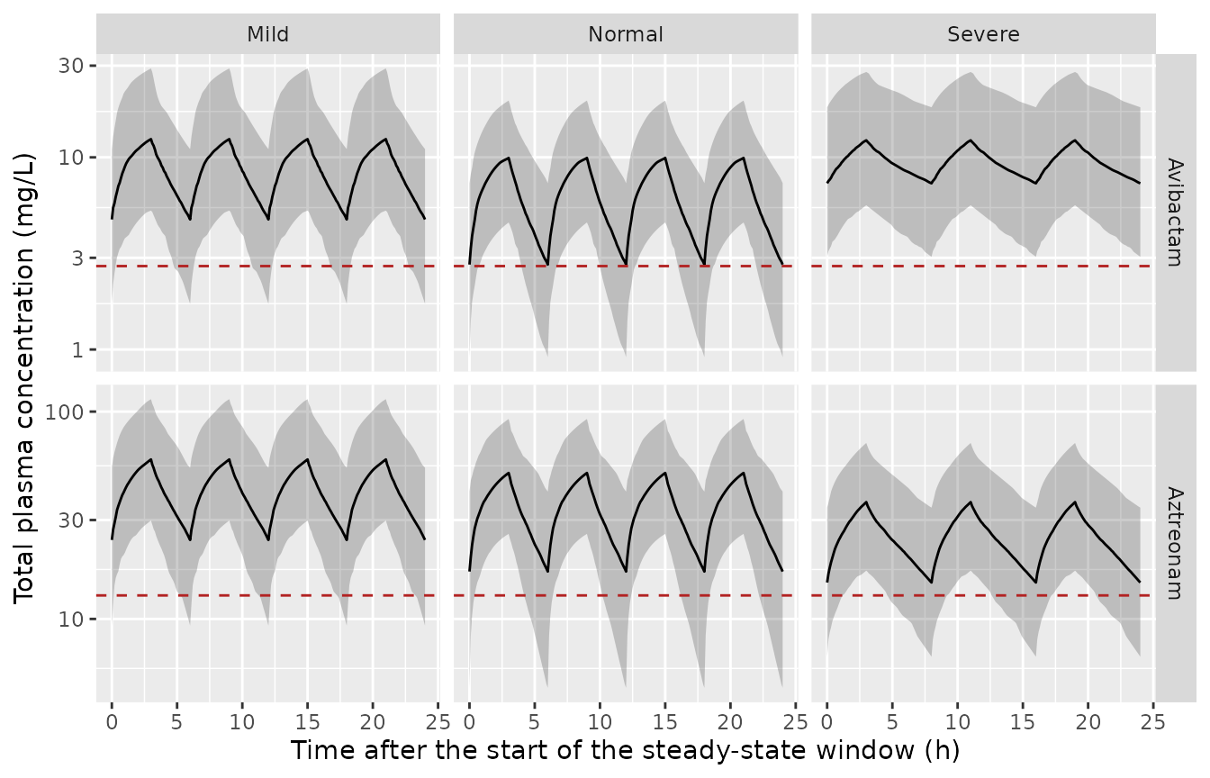

Simulated steady-state total-drug concentration-time profiles over one 24 h window by renal function group (median and 5th-95th percentiles), with the free-drug PK/PD thresholds shown on the total-drug scale.

nca_for <- function(conc_col, analyte_dose) {
  sim_nca <- sim |>
    filter(!is.na(.data[[conc_col]])) |>
    transmute(id, time, grp, Cc = .data[[conc_col]])

  dose_df <- cohort |>
    select(id, grp) |>
    left_join(arms |> select(grp, amt = all_of(analyte_dose), ii), by = "grp") |>
    tidyr::uncount(24 / ii, .id = "k") |>
    mutate(time = 216 + (k - 1) * ii) |>
    select(id, time, amt, grp)

  conc_obj <- PKNCA::PKNCAconc(sim_nca, Cc ~ time | grp + id,
                               concu = "mg/L", timeu = "h")
  dose_obj <- PKNCA::PKNCAdose(dose_df, amt ~ time | grp + id, doseu = "mg")

  intervals <- data.frame(start = 216, end = 240,
                          cmax = TRUE, tmax = TRUE, auclast = TRUE, cmin = TRUE)
  PKNCA::pk.nca(PKNCA::PKNCAdata(conc_obj, dose_obj, intervals = intervals))
}

nca_atm <- nca_for("Cc", "atm")
nca_avi <- nca_for("Cc_avi", "avi")

published_atm <- tibble::tribble(
  ~grp,      ~cmax, ~auclast,
  "Normal",   51.9,      838,
  "Mild",     65.0,     1094,
  "Severe",   40.3,      646
)

nlmixr2lib::ncaComparisonTable(
  simulated = nca_atm, reference = published_atm, by = "grp",
  units = c(cmax = "mg/L", auclast = "mg*h/L"), tolerance_pct = 20
) |>
  knitr::kable(
    caption = paste(
      "Aztreonam steady-state NCA vs Xie 2025 Table S9.",
      "* differs from reference by >20%."
    )
  )

Aztreonam steady-state NCA vs Xie 2025 Table S9. * differs from reference by >20%.

NCA parameter	grp	Reference	Simulated	% diff
Cmax (mg/L)	Normal	51.9	50.6	-2.5%
Cmax (mg/L)	Mild	65	58.8	-9.5%
Cmax (mg/L)	Severe	40.3	36.6	-9.2%
AUClast (mg*h/L)	Normal	838	818	-2.3%
AUClast (mg*h/L)	Mild	1090	990	-9.5%
AUClast (mg*h/L)	Severe	646	591	-8.4%

published_avi <- tibble::tribble(
  ~grp,      ~cmax, ~auclast,
  "Normal",   10.2,      158,
  "Mild",     13.8,      229,
  "Severe",   13.0,      237
)

nlmixr2lib::ncaComparisonTable(
  simulated = nca_avi, reference = published_avi, by = "grp",
  units = c(cmax = "mg/L", auclast = "mg*h/L"), tolerance_pct = 20
) |>
  knitr::kable(
    caption = paste(
      "Avibactam steady-state NCA vs Xie 2025 Table S9.",
      "* differs from reference by >20%."
    )
  )

Avibactam steady-state NCA vs Xie 2025 Table S9. * differs from reference by >20%.

NCA parameter	grp	Reference	Simulated	% diff
Cmax (mg/L)	Normal	10.2	9.93	-2.6%
Cmax (mg/L)	Mild	13.8	12.4	-9.9%
Cmax (mg/L)	Severe	13	12.3	-5.7%
AUClast (mg*h/L)	Normal	158	152	-3.8%
AUClast (mg*h/L)	Mild	229	207	-9.5%
AUClast (mg*h/L)	Severe	237	225	-5.3%

No row exceeds the 20% tolerance. Two aggregation caveats are worth stating explicitly rather than leaving implicit: ncaComparisonTable() summarises the simulated side by the median whereas Table S9 reports geometric means (for a log-normal quantity these coincide, so the effect here is small), and the cohort’s covariate distribution is an approximation of the paper’s unpublished multivariate-normal sampling. The severe-impairment arm is the weakest of the three for exactly that reason – the nCrCL band 15-30 is wide relative to the steep power arm that governs clearance there.

Joint probability of target attainment

The paper’s decision criterion is the joint target: free aztreonam above 8 mg/L for at least 60% of the dosing interval and free avibactam above 2.5 mg/L for at least 50%, achieved simultaneously in the same patient.

FU_ATM <- 0.616; FU_AVI <- 0.92

pta <- sim |>
  group_by(grp, id) |>
  summarise(
    fT_atm = 100 * mean(Cc     * FU_ATM > 8),
    fT_avi = 100 * mean(Cc_avi * FU_AVI > 2.5),
    .groups = "drop"
  ) |>
  group_by(grp) |>
  summarise(
    "Median %fT>8 (ATM)"   = round(median(fT_atm), 1),
    "Median %fT>2.5 (AVI)" = round(median(fT_avi), 1),
    "Joint PTA % (simulated)" = round(100 * mean(fT_atm >= 60 & fT_avi >= 50), 1),
    .groups = "drop"
  ) |>
  left_join(
    tibble::tibble(grp = c("Normal", "Mild", "Severe"),
                   "Joint PTA % (Xie 2025 Table 5)" = c(96.7, 99.3, 91.2)),
    by = "grp"
  ) |>
  rename("Renal function" = grp)

knitr::kable(pta, caption = "Joint PTA at steady state in simulated cIAI patients.")

Joint PTA at steady state in simulated cIAI patients.

Renal function	Median %fT>8 (ATM)	Median %fT>2.5 (AVI)	Joint PTA % (simulated)	Joint PTA % (Xie 2025 Table 5)
Mild	100	100	99.5	99.3
Normal	100	100	96.0	96.7
Severe	100	100	89.5	91.2

The normal-renal-function and mild-impairment arms reproduce the published joint PTA to within about one percentage point. The severe-impairment arm comes out several points low, consistent with the same covariate-sampling limitation seen in its NCA row; the published median %fT values of 100% for both drugs are reproduced in every arm.

stopifnot(
  abs(pta$`Joint PTA % (simulated)`[pta$`Renal function` == "Normal"] - 96.7) < 3,
  abs(pta$`Joint PTA % (simulated)`[pta$`Renal function` == "Mild"]   - 99.3) < 3,
  all(pta$`Median %fT>8 (ATM)` >= 85)
)

Assumptions and deviations

Covariate equation forms come from the predecessor paper. Xie 2025 prints no equations. Every functional form – the hinged nCrCL relationship, the proportional X*(1 + theta) categorical effects, the ESRD term replacing rather than multiplying the nCrCL arm, and the dialysis clearance being an absolute value rather than a multiplier – is taken from Das 2024 supplementary Tables 4 and 5, which is the same author group’s immediately preceding model on the same data lineage and prints them verbatim. Each is cross-checked against Xie 2025’s own numbers in the Source trace table above, and the renal-function ladder is an end-to-end test of all of them at once.

The APACHE II covariate is encoded as a binary stratum, and the threshold is unknown. Neither Xie 2025 nor Das 2024 writes the equation. Das 2024 prints the row as CL*(1 + theta16), which is the grammar it uses for every binary population effect and not the grammar it uses for continuous covariates (which always carry the covariate symbol, as in AGE/35**theta14); a raw continuous score is also arithmetically impossible, since at a typical ICU APACHE II of 10 the factor 1 + (-0.118)*10 is negative. The model therefore carries APACHE_II_SEV as a binary indicator. The score threshold that sets the flag is not stated in any source on disk and has not been invented here. Every simulation in this vignette holds it at the 0 reference, so no reproduced value depends on the inference.

The pooled phase-2/3 residual stratum is undefined. Table S3 reports four aztreonam proportional residual magnitudes – unqualified, phase 2, phase 3, and “phase 2/3” – without saying which records constitute the fourth stratum as distinct from the other two. All four are carried so the published parameter set is complete, selected by STUDY_AZTAVI_PHASE2 / _PHASE3 / _PHASE23, with all three zero selecting the unqualified magnitude as the Phase 1 stratum (which matches Das 2024, where the strata are phase I / II / III with an additive term on phase I only). Residual error affects only the simulated observation, not the individual predictions used throughout this vignette.

ESRD avibactam exposures are ~30% below what the encoded model predicts. The renal-function ladder reproduces every non-ESRD group within 12% but overpredicts avibactam AUC24 by 34% and Cmax by 24% in ESRD, while aztreonam matches. Since aztreonam carries no ESRD or dialysis term, the gap is isolated to the avibactam ESRD / dialysis pathway. Quantitatively, the published ESRD AUC24 of 378 mg*h/L on 225 mg q12h implies an avibactam clearance of 1.19 L/h, against the 0.88 L/h the ESRD arm produces for a 70 kg cIAI patient (10.3 * (1 - 0.923) * (1 + 0.115)) – a 35% clearance difference.

It is worth being precise about what this does not show. The obvious candidate explanation – that the published ESRD simulation applies the separate dialysis clearance of 17.9 L/h, since Xie 2025 says the approved ESRD regimen “requires patients to be receiving hemodialysis, with aztreonam-avibactam to be administered after dialysis” – cannot account for it as stated: that clearance is roughly 17 times the published-implied value and would drive AUC24 to about 23 mgh/L, far below the published 378 rather than above it. Whatever the paper did, it is much closer to the ESRD arm than to the dialysis arm, and the residual 35% must come from something intermediate that is not published – a time-weighted contribution of intermittent dialysis sessions, residual renal function in the simulated ESRD cohort, or a covariate distribution differing from the 70 kg reference patient used here. Neither the dialysis schedule nor the session duration is reported, so the sub-model is encoded as a subject-level flag (RRT_HEMODIAL_STATUS) rather than a time-varying per-session gate, and the intradialytic / interdialytic sawtooth cannot be reproduced. Nothing was tuned to close this gap, and the ladder-assert chunk asserts the ESRD row stays* an outlier so that a future change which silently closes it is noticed.

Body-weight allometry is applied to the dialysis clearance. Xie 2025 states that body weight is a structural covariate on “aztreonam and avibactam CL, Vc, Vp, and Q” without excepting the dialysis clearance, so the allometric term is applied uniformly. If the authors instead held CL_AVI_DIAL at an absolute value, predictions for dialysis patients away from 70 kg would differ.

Covariate distributions are approximations. Xie 2025 sampled weight, BSA and CrCL from a multivariate normal with a covariance matrix estimated from the analysis data set and truncated to observed ranges; that matrix is not published. This vignette samples body weight log-normally about the pooled median of 74 kg (CV 25%, truncated to the observed 33-130 kg) and nCrCL uniformly within each renal-function band, independently. The bands themselves are the paper’s raw-CrCL group boundaries used directly as nCrCL bands, i.e. assuming a body surface area of 1.73 m^2; the renal-function ladder above avoids this assumption entirely by inverting the model for the implied nCrCL instead.

Infection-type indicators are set to cIAI throughout. This follows the paper, whose dose-selection simulations were all run in cIAI patients as the most conservative case. STUDY_CIAI_PH2 is zero everywhere, as it is for every aztreonam-avibactam subject.

Observation rows use the observable name in cmt. This model declares two endpoints, so rxode2 maps Cc and Cc_avi to modelled compartments 5 and 6 and requires those names on observation records; cmt = "central" fails with 'dvid'->'cmt' ... on a undefined compartment regardless of useLinCmt. The four ODE states retain slots 1-4, so this does not trigger the slot-renumbering problem that the same syntax causes in single-endpoint models.

Free concentrations use fixed unbound fractions. The 0.616 (aztreonam) and 0.92 (avibactam) unbound fractions are conversion constants applied downstream of the PK model, not fitted parameters, so they live in the model’s population metadata rather than in ini() and are applied in this vignette.