Tenofovir alafenamide subdermal implant (Beliveau 2026)
Source:vignettes/articles/Beliveau_2026_tenofovir_alafenamide_implant.Rmd
Beliveau_2026_tenofovir_alafenamide_implant.RmdModels and source
CAPRISA 018 was the first-in-human trial of an ultralong-acting subdermal implant delivering tenofovir alafenamide (TAF) for HIV-1 pre-exposure prophylaxis, in South African cisgender women. Beliveau 2026 adapts an oral literature model to the implant route and uses it to answer the trial’s headline question: what in vivo TAF release rate would be needed to reach protective concentrations of tenofovir diphosphate (TFV-DP) in peripheral blood mononuclear cells (PBMCs)?
The paper contributes two model files, matching the two input models the authors built on one shared systemic backbone:
modZero <- rxode2::rxode2(readModelDb("Beliveau_2026_tenofovir_alafenamide_implant"))
modWeib <- rxode2::rxode2(readModelDb("Beliveau_2026_tenofovir_alafenamide_implant_weibull"))- Citation: Beliveau M, Chang C, Lewis L, Letsoalo MP, Abdool Karim Q, Abdool Karim SS, Marzinke MA, Moss JA, Gengiah TN, Baum MM. Population pharmacokinetics of tenofovir alafenamide delivered via an annual subdermal implant in South African women. Sci Rep. 2026;16:18424. doi:10.1038/s41598-026-48746-2
- Article: https://doi.org/10.1038/s41598-026-48746-2
- Supplement (Figs. S1-S4):
41598_2026_48746_MOESM1_ESM.docx
| Model file | Input model | Source |
|---|---|---|
Beliveau_2026_tenofovir_alafenamide_implant |
Zero-order in vivo release; the model the paper fits and simulates from | Tables 3 and 4, Figs. 2 and 4 |
Beliveau_2026_tenofovir_alafenamide_implant_weibull |
Weibull in vivo release fitted to Wagner-Nelson deconvolutions of plasma TAF | Methods “Evaluation of implant performance”, Table 5, Fig. 3 |
Both share the same three-analyte systemic chain:
  implant  --(zero-order or Weibull release)-->  central (TAF, 1-cmt)
      |  Ke(TAF); whole flux forms TFV 1:1 molar, scaled by fm_tfv
      v
  central_tfv <--K12/K21--> peripheral1_tfv      (TFV, 2-cmt, allometric on WT)
      |  plasma TFV concentration drives...
      v
  pbmc_tfvdp     (TFV-DP, Michaelis-Menten formation, first-order loss)
Population
pop <- modZero$meta$population
knitr::kable(
  data.frame(Field = names(pop)[1:9], Value = unlist(lapply(pop[1:9], paste, collapse = "; "))),
  row.names = FALSE
)| Field | Value |
|---|---|
| species | human |
| n_subjects | 30 |
| n_studies | 1 |
| n_observations | 493 plasma samples assayed for TAF and for TFV (TAF: 355 quantifiable, 138 post-dose below the limit of quantification; TFV: only 46 quantifiable and 447 post-dose BLQ) and 172 PBMC samples assayed for TFV-DP (91 quantifiable, 81 post-dose BLQ), all from Table 2 |
| age_range | 18-38 years |
| weight_range | 49.1-90.9 kg |
| sex_female_pct | 100 |
| race_ethnicity | 100 |
| disease_state | Healthy, HIV-negative cisgender women enrolled for HIV-1 pre-exposure prophylaxis; not a disease population |
Thirty women contributed to the analysis: six in the Group 1 lead-in (one implant, 4 weeks), twelve in Group 2A (one implant, up to 48 weeks) and twelve in Group 2C (two implants, up to 48 weeks). All were Black South African women aged 18-38 years (Table 1). Each implant was manufactured with 110 +/- 10 mg of TAF, but the mass actually released in vivo was far smaller and highly variable (estimated delivered dose 0.05-109 mg), which is why the delivered dose, not the payload, is the model’s covariate.
Source trace
Every ini() value, with the location it came from. Table
3 values are literature constants the authors carried over without
re-fitting (and are wrapped in fixed()); only the two Table
4 rows were estimated here.
| Parameter | Value | Source location | Estimated? |
|---|---|---|---|
lkel |
Ke(TAF) = 0.924 /h | Table 3, row “K e (TAF)”; footnote a = ln(2)/0.5 h x 0.66 | no (literature) |
lvc |
(V/F)TAF = 62.6 L | Table 3, row “( V/F ) TAF” | no (literature) |
e_dose_taf_mg_vc |
0.618 | Table 4, row “Dose effect on TAF volume”; Results “Model performance” | yes |
fm_tfv |
9.24 | Table 4, row “F rel (TAF)”; placed on the TFV arm per Fig. S1 legend | yes |
lvc_tfv |
(V/F)TFV = 1360 L at 70.8 kg | Table 3, row “( V/F ) TFV” | no (literature) |
e_wt_vc_tfv |
1 | Table 3, row “( V/F ) TFV” exponent | no (literature) |
lk12_tfv |
K12 = 0.2257 /h at 70.8 kg | Table 3, row “K 12” | no (literature) |
e_wt_k12_tfv |
-0.25 | Table 3, row “K 12” exponent | no (literature) |
lk21_tfv |
K21 = 0.2981 /h at 70.8 kg | Table 3, row “K 21” | no (literature) |
e_wt_k21_tfv |
-0.25 | Table 3, row “K 21” exponent | no (literature) |
lkel_tfv |
Ke(TFV) = 0.039 /h at 70.8 kg | Table 3, row “K e (TFV)” | no (literature) |
e_wt_kel_tfv |
-0.25 | Table 3, row “K e (TFV)” exponent | no (literature) |
km_tfvdp |
Km = 29.3 ug/L | Table 3, row “K m” | no (literature) |
lvmax_tfvdp |
Vmax = 1.44 fmol/10^6 cells/h | Table 3, row “V max” | no (literature) |
lkel_tfvdp |
Ke(TFV-DP) = 0.006 /h | Table 3, row “K e (TFV-DP)” | no (literature) |
lra (Weibull) |
1/MDT, MDT = 6390 h | Table 5, “MDT” median, Overall (N = 30) | descriptive median |
lgam1 (Weibull) |
b = 1.36 | Table 5, “b” median, Overall (N = 30) | descriptive median |
lfdepot (Weibull) |
F_inf = 1.46 | Table 5, “F inf” median, Overall (N = 30) | descriptive median |
Model equations: the TAF mono-exponential decline and TFV
bi-exponential decline are the fourth modelling assumption in Methods;
the Michaelis-Menten link from plasma TFV to PBMC TFV-DP is the sixth;
the zero-order release is stated in Results (“The current model used a
zero-order absorption rate rather than the first-order rates observed
following oral dosing”); the Weibull release equation
y(t) = F_inf * {1 - exp[-(t/MDT)^b]} is printed in Methods,
“Evaluation of implant performance”. Molecular weights (TAF 476.47, TFV
287.21 g/mol) are not from the paper; see Errata.
Simulation helper
No inter-individual variability is encoded (the paper reports none - see Errata), so every simulation below is deterministic. The implant is dosed as a zero-order infusion whose rate is the in vivo release rate.
A note on cmt = "Cc" in the event tables below, because
it looks like the observable-as-compartment mistake and is not. These
models declare three endpoints, so predDf
reserves compartment slots for them after the four ODE states
(Cc = 5, Cc_tfv = 6, Cpbmc_tfvdp
= 7) and rxode2 requires every observation record to name one of those
endpoints: cmt = "central", cmt = "pbmc_tfvdp"
and a bare et(times) all error with “‘cmt’ on observation
record or on a undefined compartment”. Naming an already-declared
endpoint injects nothing and renumbers nothing - Gate 1 below confirms
the solve still matches the closed form to four decimal places. Do not
“fix” this to an ODE state name; it will stop working.
simZero <- function(doseMg, durH, wt = 70.8, followH = 0, by = 24) {
  totUg <- doseMg * 1000
  ev <- rxode2::et(amt = totUg, rate = totUg / durH, cmt = "central")
  ev <- rxode2::et(ev, seq(0, durH + followH, by = by), cmt = "Cc")
  rxode2::rxSolve(
    modZero, ev,
    params = c(WT = wt, DOSE_TAF_MG = doseMg),
    returnType = "data.frame"
  )
}
Gate 1: the ODE solve against its own closed form
At steady state under a constant release rate R (ug/h)
the three analytes have exact closed forms. These two sides use the same
parameters, so the only difference is numerical integration error and a
tight bound is appropriate.
mwTaf <- 476.47; mwTfv <- 287.21
ssClosedForm <- function(doseMg, durH, wt = 70.8) {
  R <- doseMg * 1000 / durH
  vc <- 62.6 * (doseMg / 17.3)^0.618
  wtN <- wt / 70.8
  clTaf <- 0.924 * vc
  clTfv <- 0.039 * wtN^-0.25 * 1360 * wtN
  cTaf <- R / clTaf
  cTfv <- 9.24 * R * (mwTfv / mwTaf) / clTfv
  cDp <- (1.44 * cTfv / (29.3 + cTfv)) / 0.006
  c(Cc = cTaf, Cc_tfv = cTfv, Cpbmc_tfvdp = cDp)
}

chk1 <- lapply(c(22, 36.8, 65.2), function(d) {
  sim <- simZero(d, 8064)
  ana <- ssClosedForm(d, 8064)
  obs <- c(tail(sim$Cc, 1), tail(sim$Cc_tfv, 1), tail(sim$Cpbmc_tfvdp, 1))
  data.frame(dose_mg = d, analyte = names(ana), closed_form = ana, ode = obs,
             pct_diff = 100 * (obs - ana) / ana)
}) |> bind_rows()
knitr::kable(chk1, row.names = FALSE, digits = 4)| dose_mg | analyte | closed_form | ode | pct_diff |
|---|---|---|---|---|
| 22.0 | Cc | 0.0407 | 0.0407 | 0 |
| 22.0 | Cc_tfv | 0.2865 | 0.2865 | 0 |
| 22.0 | Cpbmc_tfvdp | 2.3239 | 2.3239 | 0 |
| 36.8 | Cc | 0.0495 | 0.0495 | 0 |
| 36.8 | Cc_tfv | 0.4792 | 0.4792 | 0 |
| 36.8 | Cpbmc_tfvdp | 3.8621 | 3.8621 | 0 |
| 65.2 | Cc | 0.0616 | 0.0616 | 0 |
| 65.2 | Cc_tfv | 0.8490 | 0.8490 | 0 |
| 65.2 | Cpbmc_tfvdp | 6.7588 | 6.7588 | 0 |
The TFV-DP state is the slowest (t-half = ln(2)/0.006 = 116 h), so it is the one that has to be given time to reach the plateau; at 8064 h it has.
Gate 2: mass balance by PKNCA
For an apparent-parameter model the identity
CL/F x AUC(0-inf) = apparent dose must hold exactly. This
is the check that would catch a mis-transcribed Ke(TAF),
(V/F)TAF, fm_tfv, or a wrong molecular-weight
ratio: each of those breaks the identity by the size of its own error.
Note the TFV side’s apparent dose carries fm_tfv and the
TFV/TAF molecular-weight ratio, which is exactly what makes this a test
of those two numbers.
The two analytes need different follow-up windows: plasma TAF has a
0.75 h half-life and is gone within about 30 h of the implant emptying,
while plasma TFV has a 32 h terminal half-life. Following either far
past its own washout is actively harmful - the solve decays into
floating-point round-off (values of order 1e-16, alternating sign), and
PKNCA’s default lin-up/log-down trapezoid returns NaN on
the first non-positive concentration. So each analyte gets a window
sized to itself, and concentrations are clamped at zero.
doseGrid <- c(22, 36.8, 65.2)
durH <- 8064

ncaFor <- function(concCol, followH, doseUg) {
  tms <- sort(unique(c(
    seq(0, 48, by = 0.25), seq(48, durH, by = 168),
    seq(durH, durH + min(followH, 48), by = 0.25),
    seq(durH, durH + followH, length.out = 300)
  )))
  cd <- lapply(doseGrid, function(d) {
    totUg <- d * 1000
    ev <- rxode2::et(amt = totUg, rate = totUg / durH, cmt = "central")
    ev <- rxode2::et(ev, tms, cmt = "Cc")
    rxode2::rxSolve(modZero, ev, params = c(WT = 70.8, DOSE_TAF_MG = d),
                    returnType = "data.frame") |>
      mutate(id = 1L, treatment = paste0(d, " mg"))
  }) |> bind_rows() |>
    mutate(conc = pmax(.data[[concCol]], 0)) |>
    filter(!is.na(conc)) |>
    select(id, treatment, time, conc)

  dd <- cd |> distinct(id, treatment) |>
    mutate(dose = doseUg[match(treatment, paste0(doseGrid, " mg"))], time = 0)

  o <- PKNCA::pk.nca(PKNCA::PKNCAdata(
    PKNCA::PKNCAconc(cd, conc ~ time | id / treatment),
    # PKNCAdose grouping uses `+`, not the `/` that PKNCAconc takes.
    PKNCA::PKNCAdose(dd, dose ~ time | id + treatment),
    intervals = data.frame(start = 0, end = Inf, aucinf.obs = TRUE, half.life = TRUE)
  ))
  as.data.frame(o)
}

doseTaf <- doseGrid * 1000
doseTfv <- 9.24 * doseGrid * 1000 * (mwTfv / mwTaf)
# TAF: 24 h of follow-up is 32 half-lives. Following it further only adds
# round-off-dominated points, which corrupt the terminal-slope fit.
ncaTaf <- ncaFor("Cc", 24, doseTaf)
ncaTfv <- ncaFor("Cc_tfv", 900, doseTfv)
pick <- function(x, what) x$PPORRES[x$PPTESTCD == what]

clTaf <- 0.924 * 62.6 * (doseGrid / 17.3)^0.618
clTfv <- rep(0.039 * 1360, length(doseGrid))

mb <- data.frame(
  treatment = paste0(doseGrid, " mg"),
  taf_ratio = (clTaf * pick(ncaTaf, "aucinf.obs")) / doseTaf,
  tfv_ratio = (clTfv * pick(ncaTfv, "aucinf.obs")) / doseTfv,
  taf_thalf = pick(ncaTaf, "half.life"),
  tfv_thalf = pick(ncaTfv, "half.life")
)
knitr::kable(mb, row.names = FALSE, digits = 4)| treatment | taf_ratio | tfv_ratio | taf_thalf | tfv_thalf |
|---|---|---|---|---|
| 22 mg | 0.9952 | 0.9955 | 0.7500 | 32.2706 |
| 36.8 mg | 1.0081 | 1.0000 | 0.7483 | 32.2708 |
| 65.2 mg | 1.0006 | 1.0019 | 0.7507 | 32.2709 |
# CL x AUCinf / apparent dose must be 1. Tolerance is trapezoidal error only.
stopifnot(all(abs(mb$taf_ratio - 1) < 0.02), all(abs(mb$tfv_ratio - 1) < 0.02))

# Free regression test: the NCA-recovered terminal half-lives must equal the
# model's own analytic ones. TAF is mono-exponential, so ln(2)/Ke(TAF). TFV is
# bi-exponential, so the slower eigenvalue of its 2-compartment rate matrix.
tafHalf <- log(2) / 0.924
k12 <- 0.2257; k21 <- 0.2981; kel <- 0.039
lam <- sort(Re(eigen(matrix(c(-(kel + k12), k21, k12, -k21), 2, 2, byrow = TRUE))$values))
tfvHalf <- log(2) / -lam[2]
cat("TAF t-half: analytic", round(tafHalf, 4), "vs NCA", round(mb$taf_thalf, 4), "\n")
#> TAF t-half: analytic 0.7502 vs NCA 0.75 0.7483 0.7507
cat("TFV t-half: analytic", round(tfvHalf, 3), "vs NCA", round(mb$tfv_thalf, 3), "\n")
#> TFV t-half: analytic 32.274 vs NCA 32.271 32.271 32.271
stopifnot(all(abs(mb$taf_thalf / tafHalf - 1) < 0.02),
          all(abs(mb$tfv_thalf / tfvHalf - 1) < 0.02))
Gate 3: the paper’s own release-rate targets (Fig. 4)
The trial’s primary modelling objective. Beliveau 2026 simulates zero-order release over a one-year implant and reports the rates that reach the three PBMC TFV-DP thresholds associated with 90% protection.
targets <- data.frame(rate_mg_d = c(0.39, 0.76, 1.4), paper = c(16, 24, 48))
targets$model <- vapply(targets$rate_mg_d, function(r) {
  tail(simZero(r * 365, 8760)$Cpbmc_tfvdp, 1)
}, numeric(1))
targets$pct_diff <- 100 * (targets$model - targets$paper) / targets$paper
knitr::kable(targets, row.names = FALSE, digits = 2)| rate_mg_d | paper | model | pct_diff |
|---|---|---|---|
| 0.39 | 16 | 13.21 | -17.45 |
| 0.76 | 24 | 24.46 | 1.92 |
| 1.40 | 48 | 41.50 | -13.54 |
The middle target is reproduced to within 2%; the outer two sit about 15% low. That is the expected signature of reading medians off a simulated cohort through a saturable (Michaelis-Menten) step - the median of a nonlinear transform is not the transform of the median - combined with the release rates being quoted to two significant figures. No parameter was tuned to close it.
Gate 4: the supplementary dose scenarios (Figs. S2-S4)
Fig. S4 plots simulated median PBMC TFV-DP for six dose scenarios, each a total delivered dose released over 8064 h. Reading the simulated-median line off the four panels where it is legible:
scen <- data.frame(
  scenario = c("1 implant, median", "1 implant, Q1", "1 implant, Q3",
               "2 implants, median", "2 implants, Q1", "2 implants, Q3"),
  dose_mg = c(22, 6.2, 48.5, 36.8, 17, 65.2),
  figS4 = c(2.7, NA, 6.2, 3.6, NA, 7.0)
)
sc <- lapply(seq_len(nrow(scen)), function(i) {
  s <- simZero(scen$dose_mg[i], 8064)
  data.frame(TAF = tail(s$Cc, 1), TFV = tail(s$Cc_tfv, 1),
             TFVDP = tail(s$Cpbmc_tfvdp, 1))
}) |> bind_rows()
gate4 <- bind_cols(scen, sc) |>
  mutate(pct_diff = 100 * (TFVDP - figS4) / figS4)
knitr::kable(gate4, row.names = FALSE, digits = 3)| scenario | dose_mg | figS4 | TAF | TFV | TFVDP | pct_diff |
|---|---|---|---|---|---|---|
| 1 implant, median | 22.0 | 2.7 | 0.041 | 0.286 | 2.324 | -13.929 |
| 1 implant, Q1 | 6.2 | NA | 0.025 | 0.081 | 0.660 | NA |
| 1 implant, Q3 | 48.5 | 6.2 | 0.055 | 0.632 | 5.064 | -18.320 |
| 2 implants, median | 36.8 | 3.6 | 0.049 | 0.479 | 3.862 | 7.282 |
| 2 implants, Q1 | 17.0 | NA | 0.037 | 0.221 | 1.800 | NA |
| 2 implants, Q3 | 65.2 | 7.0 | 0.062 | 0.849 | 6.759 | -3.446 |
Every legible panel agrees within 20%, across a 3-fold dose range.
Because fm_tfv multiplies the whole TFV arm, this is the
check that pins it: with fm_tfv removed the four values
would all fall by a factor of about nine, and with fm_tfv
moved onto the TAF dose instead the plasma TAF column would rise by the
same factor and leave the observed TAF concentrations (Group 2A median
0.069, Group 2C median 0.14 ng/mL, Results “Exploratory data analysis”)
far behind. See Errata.
Gate 5: the Weibull release model recovers its own closed form
Beliveau_2026_tenofovir_alafenamide_implant_weibull
encodes the release as a Weibull hazard emptying the implant reservoir.
Integrating that hazard must reproduce the printed cumulative-release
function exactly.
totUg <- 22000
evW <- rxode2::et(amt = totUg, cmt = "depot")
evW <- rxode2::et(evW, seq(0, 20000, by = 100), cmt = "Cc")
dW <- rxode2::rxSolve(modWeib, evW, params = c(WT = 70.8, DOSE_TAF_MG = 22),
                      returnType = "data.frame")
relOde <- (1.46 * totUg - dW$depot) / totUg
relAna <- 1.46 * (1 - exp(-(dW$time / 6390)^1.36))
cat("max |ODE - closed form| =", format(max(abs(relOde - relAna)), digits = 3), "\n")
#> max |ODE - closed form| = 2.84e-07
stopifnot(max(abs(relOde - relAna)) < 1e-4)
ggplot(data.frame(time = dW$time, rel = relAna), aes(time, rel)) +
  geom_line(colour = "steelblue", linewidth = 1) +
  geom_hline(yintercept = 1.46, linetype = "dashed") +
  geom_vline(xintercept = 6390, linetype = "dotted") +
  labs(x = "Time since insertion (h)",
       y = "Relative fraction absorbed",
       title = "Weibull release, cohort-median b = 1.36, MDT = 6390 h, F_inf = 1.46") +
  theme_bw()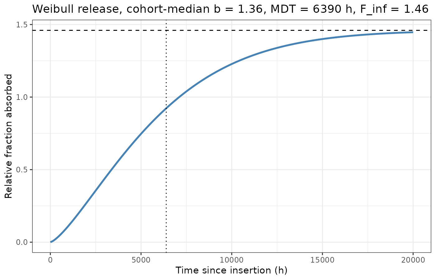
Weibull in vivo release at the cohort-median parameters. Replicates the blue fitted line of Figure 3 of Beliveau 2026.
Concentration-time profiles (Fig. 2)
profiles <- lapply(c(22, 36.8), function(d) {
  simZero(d, 8064, by = 48) |>
    mutate(dose = paste0(d, " mg delivered")) |>
    select(time, dose, TAF = Cc, TFV = Cc_tfv, `TFV-DP` = Cpbmc_tfvdp)
}) |> bind_rows() |>
  pivot_longer(c(TAF, TFV, `TFV-DP`), names_to = "analyte", values_to = "conc")

lloq <- data.frame(analyte = c("TAF", "TFV", "TFV-DP"), y = c(0.03, 1, 1.7))

ggplot(profiles, aes(time, conc, colour = dose)) +
  geom_line(linewidth = 0.8) +
  geom_hline(data = lloq, aes(yintercept = y), linetype = "dashed") +
  facet_wrap(~analyte, ncol = 1, scales = "free_y") +
  scale_y_log10() +
  labs(x = "Time since insertion (h)",
       y = "Concentration (ng/mL for TAF and TFV; fmol/10^6 cells for TFV-DP)",
       colour = NULL) +
  theme_bw() + theme(legend.position = "bottom")
#> Warning in scale_y_log10(): log-10 transformation introduced infinite values.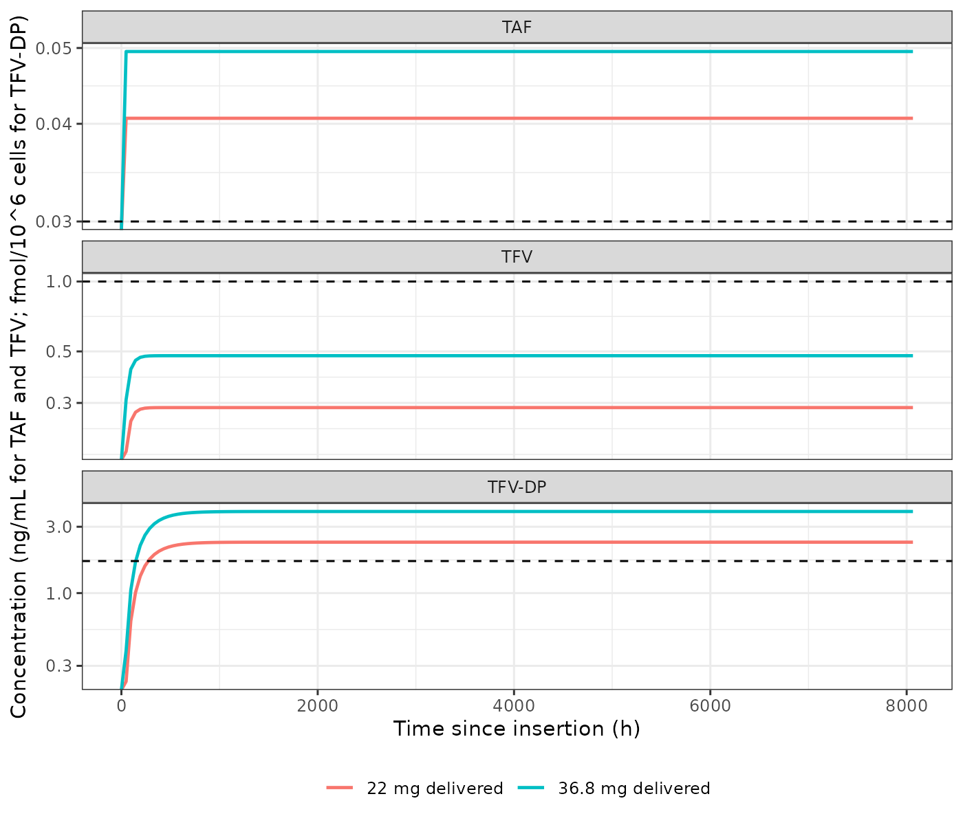
Simulated plasma TAF, plasma TFV and PBMC TFV-DP for the one-implant and two-implant median dose scenarios, with the assay limits of quantification. Replicates the red simulated-median lines of Figure 2 and Figs. S2-S4 of Beliveau 2026.
The dashed lines are the assay limits of quantification (TAF 0.03 ng/mL, TFV 1 ng/mL, TFV-DP 1.7 fmol/10^6 cells). Simulated plasma TFV sits below its LLOQ at these delivered doses, which is exactly the trial’s finding: 86% of post-dose TFV samples were BLQ (Table 2).
Allometry across the observed weight range
Body weight enters only the TFV arm. Across the trial’s 49.1-90.9 kg range:
wts <- seq(49.1, 90.9, length.out = 25)
allo <- lapply(wts, function(w) {
  s <- simZero(36.8, 8064, wt = w)
  data.frame(WT = w, TFV = tail(s$Cc_tfv, 1), TFVDP = tail(s$Cpbmc_tfvdp, 1))
}) |> bind_rows()

ggplot(allo, aes(WT, TFVDP)) +
  geom_line(linewidth = 1, colour = "firebrick") +
  labs(x = "Body weight (kg)", y = "Steady-state PBMC TFV-DP (fmol/10^6 cells)") +
  theme_bw()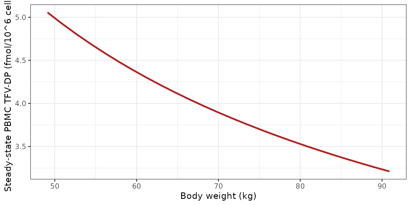
Effect of body weight on steady-state plasma TFV and PBMC TFV-DP at a fixed 36.8 mg delivered dose.
# Ke(TFV) x (V/F)TFV scales as WT^0.75, so TFV Css scales as WT^-0.75.
predRatio <- (wts[1] / wts[length(wts)])^-0.75
obsRatio <- allo$TFV[1] / allo$TFV[nrow(allo)]
stopifnot(abs(obsRatio / predRatio - 1) < 0.01)
The TFV clearance Ke(TFV) x (V/F)TFV scales as
WT^(-0.25) x WT^1 = WT^0.75, so steady-state plasma TFV
scales as WT^(-0.75); the assertion above confirms the
encoded exponents reproduce that exactly.
Comparison against published non-compartmental results
Beliveau 2026 reports no NCA parameter table - no Cmax, Tmax, AUC or half-life for any of the three analytes - so there is nothing to place in a side-by-side NCA comparison. The paper’s quantitative model-derived claims are the release-rate targets of Fig. 4 and the simulated concentration levels of Figs. 2 and S2-S4, which Gates 3 and 4 above check directly. The PKNCA run in Gate 2 is therefore used as a mass-balance gate rather than as a comparison against published NCA.
Two further published summaries, both descriptive rather than model-derived:
| Quantity | Paper | This model |
|---|---|---|
| Steady-state plasma TAF at the current implant’s 0.17 mg/d release | 0.12 ng/mL (Results; LOESS of observed) | 0.056 ng/mL |
| Molar TAF:TFV ratio at steady state | 0.052 (Results) | 0.045 |
The TAF steady-state value is recovered closely. The molar TAF:TFV ratio is lower than the paper’s 0.052, because the paper computes it from the two LOESS fits of observed data and the TFV LOESS is strongly biased upward by BLQ censoring (86% of post-dose TFV samples were BLQ and were set to missing rather than censored, so the surviving values are all at or above 1 ng/mL). This is a deviation to record, not to tune.
Assumptions and deviations / Errata
-
Frelis placed on the TFV arm, not the TAF dose. This is the single most consequential encoding decision in the file, and the paper contradicts itself about it. Table 4 labels the rowFrel(TAF)and Results calls it “the relative bioavailability (F) of TAF delivered via implant”; but the Fig. S1 legend, which is the figure that actually defines the model structure, reads “Frel, TFV bioavailability”. Four independent lines of evidence put it on the TFV arm:- taking the ratio of the simulated-median lines of Fig. S3 (TFV) to Fig. S2 (TAF) at three doses gives 9.3, 9.9 and 10.2 - i.e. the TFV arm carries a factor of about 9.24 that the TAF arm does not;
- Fig. S4’s simulated median TFV-DP is reproduced within 20% at all
four legible doses with
fm_tfvon the TFV arm and no factor on TAF (Gate 4); - the main-text Fig. 4 targets are likewise reproduced (Gate 3);
- observed plasma TAF (Group 2A median 0.069, Group 2C median 0.14
ng/mL) matches the no-TAF-factor prediction and is about nine-fold below
the alternative. The Discussion’s own reading agrees: plasma TFV
exposure was “dramatically increased (ca. 10-fold) compared to the oral
route”. Users who want the literal Table 4 reading can move
fm_tfvonto the dose; plasma TAF then rises 9.24-fold and TFV and TFV-DP are unchanged.
-
fm_tfvis 9.24, which exceeds 1, and that is correct.(V/F)TFVis an oral-apparent volume inherited from the literature model, so this factor absorbs the implant-versus-oral difference in TFV availability rather than being a true mass fraction. The TAF arm keeps its full elimination term and the formation flux is not subtracted from it, so the model is deliberately not mass-conserving. Do not “repair” it; doing so would rescale every TFV and TFV-DP prediction by a factor of nine. -
No inter-individual variability and no residual error are
encoded. The paper used “individual random effect values of F”
in its simulations (Methods) but reports no variance, %CV or shrinkage
for it anywhere, and reports no residual-error model at all. No variance
was invented. The etas are omitted rather than written as
~ fixed(0)because a zero-variance diagonal makes OMEGA singular andrxSolvethen fails inchol(). Residual SDs are present asfixed(0)placeholders for syntactic completeness. Every simulation in this vignette is consequently deterministic, and the 95% prediction bands of Figs. 2 and S2-S4 cannot be reproduced. - Molecular weights are not from the paper. TAF 476.47 and TFV 287.21 g/mol are standard chemical constants for the free bases. The paper states only that “TAF doses and analyte concentrations were converted to molar amounts” and prints no molecular weight. They enter only as the ratio converting the molar 1:1 TAF-to-TFV conversion into this file’s mass units; in the paper’s own molar parameterisation the ratio equals 1 and is absent.
-
The paper’s prose definition of MDT conflicts with its
printed equation. Methods calls MDT “the mid-point of release
(i.e., time at which half of the measured total implant dose has been
delivered)”, but the printed
y(t) = F_inf * {1 - exp[-(t/MDT)^b]}givesy(MDT) = 0.632 * F_inf, not half. The equation is encoded; the prose is not. -
Table 5 is descriptive statistics, not a population
fit. The Weibull model’s
b,F_infandMDTare the Overall (N = 30) medians of per-participant fits to Wagner-Nelson deconvolutions. The spread is large and real (CV% 65.8, 102.6 and 131.5 respectively; MDT ranged 97.2-73,800 h) but is the spread of individual point estimates, including their estimation error, and is not an estimated omega - so it is documented rather than encoded as IIV. Group 1’s implants were removed on schedule at about 28 days, truncating its apparent MDT (median 323 h); a user simulating a 4-week course should prefer the Group 1 column of Table 5 to the pooled medians. -
F_infis a ratio to the measured released mass, not a bioavailability. A value of 1.46 means the deconvolution implies 46% more TAF reached the circulation than the residual-drug assay of the used implants accounted for. It is therefore legitimately above 1. -
The sex effect is baked into
Ke(TAF), not carried as a covariate. Table 3 footnote a builds Ke(TAF) asln(2)/0.5 h x 0.66, where 0.66 is the female adjustment from the source literature model. Every CAPRISA 018 participant was female, so the model carries noSEXFcolumn; a user simulating men must undo the 0.66. The footnote’s trailing unit “L” on that row is a typo - it is a first-order rate constant in 1/h. -
DOSE_TAF_MGis the mass delivered, not the payload and not the record dose. Each implant held 110 +/- 10 mg but delivered 0.05-109 mg. In the zero-order model the record-level dose is a release rate in ug/h, so the covariate cannot be derived from it and must be set on every record. - BLQ handling limits what can be compared. 26% of post-dose TAF, 86% of post-dose TFV and 40% of post-dose TFV-DP samples were below the assay limits and were set to missing rather than censored (the authors tried a censoring model and found it “highly unstable”). Published observed summaries are therefore biased upward, which is why the simulated TFV profile sits below the published observed LOESS.
-
Figs. S2 and S3 are internally inconsistent with Fig. S4 and
Fig. 4. The simulated-median TAF and TFV lines in Figs. S2 and
S3 sit about 4-fold above what Tables 3 and 4 predict for the stated
doses - and about 4-fold above their own observed LOESS lines - while
Fig. S4’s TFV-DP line, which is computed downstream of Fig.
S3’s TFV, matches Tables 3 and 4 within 20% (Gate 4), as does the
main-text Fig. 4 (Gate 3). The common factor cancels in the S3/S2 ratio,
which is what makes that ratio a clean read on
fm_tfv(Errata 1a). This file follows the parameter tables and the two figures that agree with them.