Garadacimab (Garcia 2025)
Source:vignettes/articles/Garcia_2025_garadacimab.Rmd
Garcia_2025_garadacimab.RmdModel and source
Garcia 2025 reports three linked analyses of garadacimab, a first-in-class fully human IgG4 monoclonal antibody targeting activated factor XII (FXIIa) developed for long-term prophylaxis of hereditary angioedema (HAE) attacks. The paper is packaged here as two model files, following the author’s own structure:
-
Garcia_2025_garadacimab– the population PK model (two-compartment, first-order absorption and elimination) coupled to the population PK/PD model for FXIIa-mediated kallikrein activity (direct sigmoidal Emax inhibition). -
Garcia_2025_garadacimab_hae_attack– the exposure-response repeated-time-to-event (RTTE) model for HAE attacks, with the same PK system embedded so the attack hazard is driven by simulated garadacimab concentration.
The split mirrors the source: the PopPK/PD analysis and the ER
analysis are separate NONMEM runs (Methods S1 and Methods S2
respectively), and the ER control stream re-implements the PK ODEs in
$DES rather than sharing them.
- Citation: Garcia R, Cheng S, Glassman F, Sharma A, De Miguel-Lillo B, Wiens M, Johnston C, Lawo JP, Pragst I, French J, Polhamus D, Nandy P. Population pharmacokinetic/pharmacodynamic and exposure-response modeling of garadacimab in healthy volunteers and patients with hereditary angioedema. CPT Pharmacometrics Syst Pharmacol. 2025;14(5):954-963. doi:10.1002/psp4.70009. Open Access under CC BY-NC 4.0. Structural equations and the NONMEM control streams are in Methods S1; final parameter estimates are in Tables S4-S7 of the supplement (Wiley file PSP4-14-954-s001.docx). Sister model file from the same paper: modellib(‘Garcia_2025_garadacimab_hae_attack’).
- Article: https://doi.org/10.1002/psp4.70009
- Supplement (Methods S1/S2 control streams and Tables S1-S12): Wiley
file
PSP4-14-954-s001.docx, published with the open-access article (PMC12072213).
mod_pkpd <- rxode2::rxode2(readModelDb("Garcia_2025_garadacimab"))
mod_er   <- rxode2::rxode2(readModelDb("Garcia_2025_garadacimab_hae_attack"))
Population
The PK analysis dataset comprised 242 unique participants – healthy volunteers and patients with HAE – who received at least one dose of garadacimab prior to one evaluable PK sample. The PopPK/PD dataset for FXIIa-mediated kallikrein activity added 20 placebo recipients to those same 242 participants, and the ER dataset comprised 177 patients with HAE. Data were pooled from five studies (Table S1): two phase I studies in healthy volunteers (ACTRN 12616001438448 and the Japanese/White ethnobridging study NCT04580654), one phase II study in patients with HAE including its randomized placebo-controlled and open-label periods (NCT03712228), and two phase III studies in patients with HAE-C1INH (pivotal VANGUARD NCT04656418 and open-label extension NCT04739059).
Ages ranged from 12 to 73 years (median 41), body weight from 43.3 to 153 kg (median 79.2), and the run-in HAE attack rate from 0.13 to 3.11 attacks per week (median 0.61) (Results Section 3.1; per-study baseline characteristics in Table S3). Sex ratios were comparable across studies except the phase I study ACTRN 12616001438448, which enrolled only healthy male volunteers per protocol, so the source reports no single pooled female percentage.
str(readModelDb("Garcia_2025_garadacimab")()$population, max.level = 1)
#> List of 12
#>  $ species       : chr "human"
#>  $ n_subjects    : int 242
#>  $ n_studies     : int 5
#>  $ age_range     : chr "12-73 years (median 41)"
#>  $ weight_range  : chr "43.3-153 kg (median 79.2)"
#>  $ sex_female_pct: NULL
#>  $ race_ethnicity: NULL
#>  $ disease_state : chr "Pooled healthy volunteers and patients with hereditary angioedema due to C1-inhibitor deficiency or dysfunction"| __truncated__
#>  $ dose_range    : chr "Phase I single intravenous doses up to 10 mg/kg and subcutaneous doses; phase II subcutaneous 75, 200, or 600 m"| __truncated__
#>  $ regions       : chr "multinational"
#>  $ biomarkers    : chr "FXIIa-mediated kallikrein activity, expressed as percent of baseline (POB), measured with an in-house chromogen"| __truncated__
#>  $ notes         : chr "PK analysis dataset: 242 unique participants who received at least one dose of garadacimab prior to one evaluab"| __truncated__
Source trace
Every ini() entry carries an in-file comment naming its
source location. The table below collects them.
| Equation / parameter | Value | Source location |
|---|---|---|
| Two-compartment PK, first-order absorption/elimination | ADVAN4 TRANS4 | Methods S1, “Two-compartment PK (PopPK) model code” |
lcl (CL) |
0.00664 L/h | Table S4, final model |
lvc (V2) |
2.37 L | Table S4, final model |
lq (Q) |
0.00685 L/h | Table S4, final model |
lvp (V3) |
1.41 L | Table S4, final model |
lka (ka) |
0.00824 1/h | Table S4, final model |
logitfdepot (F1) |
0.387 | Table S4, final model |
e_wt_cl (WT on CL and Q) |
1.16 (exponent) | Table S4, final model |
e_wt_vc (WT on V2 and V3) |
0.843 (exponent) | Table S4, final model |
e_race_japanese_cl |
1.27-fold | Table S4, final model |
e_race_chinese_cl |
1.02-fold | Table S4, final model |
e_dis_hae_cl |
1.05-fold | Table S4, final model |
e_creat_cl |
-0.0343 (exponent) | Table S4, final model |
e_alt_cl |
-0.0773 (exponent) | Table S4, final model |
e_tbili_cl |
-0.136 (exponent) | Table S4, final model |
| PK IIV block (CL, V2, logit F1) | 0.175 / 0.263 / 0.717 / 0.154 / 0.174 / 0.359 | Table S5, final model |
propSd (PK proportional) |
var 0.0395 (CV% 19.9) | Table S5, final model |
| Direct sigmoidal Emax inhibition | E0 * (1 - Emax * C^g / (EC50^g + C^g)) |
Methods S1, PopPK/PD $ERROR block |
lemax (Emax) |
0.988 | Table S6, final model |
lec50 (EC50) |
17600 ng/mL | Table S6, final model |
le0 (E0) |
98.8 % of baseline | Table S6, final model |
lhill (gamma) |
2.05 | Table S6, final model |
| PD IIV block (EC50, E0, gamma) | 0.168 / 0.0148 / 0.0268 / 0.0846 / 0.0254 / 0.150 | Table S7, final model (covariance labels corrected – see Errata) |
propSd_kallikrein / addSd_kallikrein
|
var 0.0577 / var 6.01 | Table S7, final model |
Log-hazard log h = log h0 + f_placebo + f_drug
|
– | Methods S2, ER model development |
lhaz_base (h0) |
0.00440 1/h | Table S8, final model |
iplac (placebo/study effect) |
0.728 multiplicative (= 1 - 0.272) | Table S8, final model |
lec50 (hazard EC50) |
303 ng/mL | Table S8, final model |
logitimax (Imax) |
logit 7 FIX (= 0.999089) | Methods S2 $THETA(4); Table S8 “1 (fixed)” |
lhill (hazard Hill) |
1 FIX | Methods S2 $THETA(5); Table S8 “1.00 (fixed)” |
| ER IIV block (h0, EC50) | 0.206 / 0.0445 / 4.95 | Table S9, final model |
Covariate-effect scale verification
Table S4 reports the two kinds of covariate effect on
different scales: continuous covariates enter as
THETA * log(cov / ref), so the tabulated number is the
power exponent, whereas categorical covariates enter as
a THETA added in the log domain and the tabulated number is
the back-transformed fold change. Reading either row
type on the wrong scale would silently corrupt the covariate model, so
the reading is verified below by reproducing all fifteen rows of the
main-text Figure 1 forest plot, which reports steady-state exposure
relative to the reference subject. Because AUC(tau,ss) is inversely
proportional to CL, the predicted ratio is
1 / (CL ratio).
fig1 <- tibble::tribble(
  ~covariate,            ~cl_ratio,                 ~published,
  "Patient with HAE",    1.05,                      0.944,
  "Japanese",            1.27,                      0.790,
  "Chinese",             1.02,                      0.976,
  "BL weight 105 kg",    (105 / 70)^1.16,           0.624,
  "BL weight 95 kg",     (95  / 70)^1.16,           0.701,
  "BL weight 85 kg",     (85  / 70)^1.16,           0.798,
  "BL weight 75 kg",     (75  / 70)^1.16,           0.923,
  "BL weight 65 kg",     (65  / 70)^1.16,           1.09,
  "BL weight 55 kg",     (55  / 70)^1.16,           1.32,
  "BL sCr 0.6 mg/dL",    (0.6 / 0.75)^-0.0343,      0.993,
  "BL sCr 1.0 mg/dL",    (1.0 / 0.75)^-0.0343,      1.01,
  "BL bilirubin 13 umol/L", (13 / 8)^-0.136,        1.07,
  "BL bilirubin 4 umol/L",  (4  / 8)^-0.136,        0.911,
  "BL ALT 40 U/L",       (40 / 25)^-0.0773,         1.04,
  "BL ALT 10 U/L",       (10 / 25)^-0.0773,         0.930
) |>
  mutate(predicted = 1 / cl_ratio,
         `% diff`  = round(100 * (predicted - published) / published, 2),
         predicted = round(predicted, 4)) |>
  select(covariate, predicted, published, `% diff`)

knitr::kable(
  fig1 |> rename("Covariate" = covariate, "Predicted AUC ratio" = predicted,
                 "Figure 1 median" = published),
  caption = "Replicates Figure 1 of Garcia 2025: model-predicted AUC(tau,ss) relative to the reference subject.",
  align = c("l", "r", "r", "r")
)| Covariate | Predicted AUC ratio | Figure 1 median | % diff |
|---|---|---|---|
| Patient with HAE | 0.9524 | 0.944 | 0.89 |
| Japanese | 0.7874 | 0.790 | -0.33 |
| Chinese | 0.9804 | 0.976 | 0.45 |
| BL weight 105 kg | 0.6248 | 0.624 | 0.13 |
| BL weight 95 kg | 0.7017 | 0.701 | 0.10 |
| BL weight 85 kg | 0.7983 | 0.798 | 0.04 |
| BL weight 75 kg | 0.9231 | 0.923 | 0.01 |
| BL weight 65 kg | 1.0898 | 1.090 | -0.02 |
| BL weight 55 kg | 1.3228 | 1.320 | 0.21 |
| BL sCr 0.6 mg/dL | 0.9924 | 0.993 | -0.06 |
| BL sCr 1.0 mg/dL | 1.0099 | 1.010 | -0.01 |
| BL bilirubin 13 umol/L | 1.0683 | 1.070 | -0.16 |
| BL bilirubin 4 umol/L | 0.9100 | 0.911 | -0.11 |
| BL ALT 40 U/L | 1.0370 | 1.040 | -0.29 |
| BL ALT 10 U/L | 0.9316 | 0.930 | 0.17 |
Every one of the fifteen forest-plot entries is reproduced to within 0.89%, confirming both the mixed-scale reading of Table S4 and the power/log-linear covariate structure.
Virtual cohort
The dose-justification simulations in the paper sampled adult covariates from the analysis dataset and adolescent covariates from the National Health and Examination Survey, which is not reproducible from the available sources. Here a 200-subject cohort of adult patients with HAE is generated with body weight log-normally distributed to match the reported median of 79.2 kg and truncated to the reported 43.3-153 kg range; all other covariates are held at the reference values that define the source’s reference subject (non-Japanese, non-Chinese, baseline serum creatinine 0.75 mg/dL, ALT 25 U/L, bilirubin 8 umol/L).
n_sub <- 200L
tau   <- 30 * 24     # 30-day dosing interval (phase III: 30 +/- 4 days)
n_dose <- 8L

wt <- pmin(pmax(exp(rnorm(n_sub, log(79.2), 0.24)), 43.3), 153)

# Loading dose = two 200 mg SC injections, then 200 mg SC once monthly.
dose_ev <- as.data.frame(
  rxode2::et(amt = 400, cmt = "depot") |>
    rxode2::et(amt = 200, cmt = "depot", time = tau, ii = tau, addl = n_dose - 1L)
)
dose_ev$cmt  <- as.character(dose_ev$cmt)
dose_ev$dvid <- NA_integer_

# Both model outputs are algebraic, so observation rows carry a dvid and
# cmt = NA rather than naming a compartment.
obs_ev <- data.frame(
  time = seq(tau * n_dose, tau * (n_dose + 1L), by = 4),
  amt = NA_real_, evid = 0L, cmt = NA_character_,
  ii = NA_real_, addl = NA_integer_, dvid = 1L
)

one_subject <- bind_rows(
  dose_ev[, c("time", "amt", "evid", "cmt", "ii", "addl", "dvid")], obs_ev
)
one_subject <- one_subject[order(one_subject$time, -one_subject$evid), ]

events <- do.call(rbind, lapply(seq_len(n_sub), function(i) {
  x <- one_subject
  x$id <- i
  x$WT <- wt[i]
  x
}))
events$RACE_JAPANESE <- 0
events$RACE_CHINESE  <- 0
events$DIS_HAE       <- 1
events$CREAT         <- 0.75
events$ALT           <- 25
events$TBILI         <- 8
events$ON_TREATMENT  <- 1
Simulation
Typical-value PK and PD profiles
Replicates Figure 4 of Garcia 2025: model-predicted garadacimab concentration and FXIIa-mediated kallikrein activity following the loading dose of two 200 mg SC injections followed by 200 mg SC once monthly.
typ_ev <- one_subject
typ_ev$time <- typ_ev$time  # keep as-is
typ_obs <- data.frame(time = seq(0, tau * (n_dose + 1L), by = 6),
                      amt = NA_real_, evid = 0L, cmt = NA_character_,
                      ii = NA_real_, addl = NA_integer_, dvid = 1L)
typ_ev <- bind_rows(dose_ev[, c("time", "amt", "evid", "cmt", "ii", "addl", "dvid")], typ_obs)
typ_ev <- typ_ev[order(typ_ev$time, -typ_ev$evid), ]
typ_ev$WT <- 79.2; typ_ev$RACE_JAPANESE <- 0; typ_ev$RACE_CHINESE <- 0
typ_ev$DIS_HAE <- 1; typ_ev$CREAT <- 0.75; typ_ev$ALT <- 25; typ_ev$TBILI <- 8

typ <- rxode2::rxSolve(rxode2::zeroRe(mod_pkpd), typ_ev, returnType = "data.frame") |>
  filter(!is.na(Cc))
#> ℹ omega/sigma items treated as zero: 'etalcl', 'etalvc', 'etalogitfdepot', 'etalec50', 'etale0', 'etalhill'

typ |>
  transmute(day = time / 24,
            `Garadacimab (ug/mL)` = Cc / 1000,
            `FXIIa-mediated kallikrein activity (% of baseline)` = kallikrein) |>
  pivot_longer(-day) |>
  ggplot(aes(day, value)) +
  geom_line(linewidth = 0.7) +
  facet_wrap(~name, scales = "free_y", ncol = 1) +
  labs(x = "Time (days)", y = NULL) +
  theme_bw()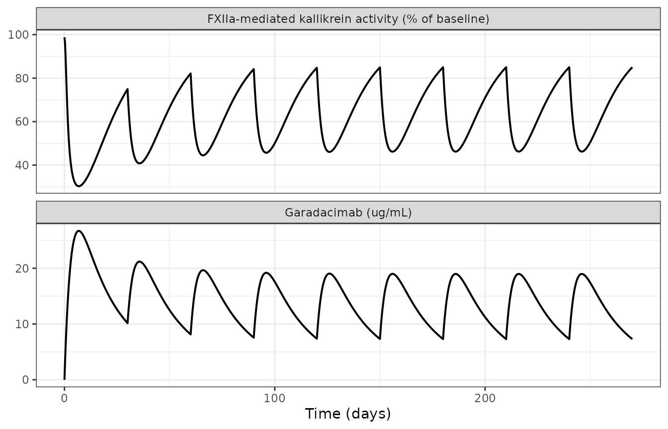
Replicates Figure 4 of Garcia 2025 (typical-value trajectories).
The typical-value trough after the loading dose is above the eventual steady-state trough, which is the source’s central dose-justification claim: the loading dose of two 200 mg injections achieves steady-state exposures from the first administration.
trough <- sapply(0:n_dose, function(k) {
  tt <- tau * k
  typ$Cc[which.min(abs(typ$time - tt))] / 1000
})
loading <- tibble::tibble(
  `Dosing interval` = paste0("Trough before dose ", seq_along(trough)),
  `Ctrough (ug/mL)` = round(trough, 2)
)
knitr::kable(head(loading, 5), caption = "Typical-value pre-dose troughs; the first-interval trough already exceeds the steady-state trough.")| Dosing interval | Ctrough (ug/mL) |
|---|---|
| Trough before dose 1 | 0.00 |
| Trough before dose 2 | 10.15 |
| Trough before dose 3 | 8.14 |
| Trough before dose 4 | 7.55 |
| Trough before dose 5 | 7.37 |
# Table S12: the probability of exceeding the 6.00 ug/mL Cmin threshold is
# HIGHER in the first dosing interval with a loading dose (0.889) than at
# steady state (0.731) -- i.e. the first-interval trough must exceed the
# steady-state trough.
stopifnot(trough[2] > trough[length(trough)], trough[2] > 6.00)PKNCA validation
Non-compartmental analysis over the final (steady-state) dosing
interval. The concentration frame is filtered only on
!is.na(Cc) so the interval-start record is retained.
nca_conc <- sim |>
  transmute(id = as.integer(id), time, conc = Cc / 1000, treatment = "200 mg SC Q30D")

conc_obj <- PKNCA::PKNCAconc(nca_conc, conc ~ time | id / treatment,
                             concu = "ug/mL", timeu = "h")
dose_obj <- PKNCA::PKNCAdose(
  data.frame(id = seq_len(n_sub), time = tau * n_dose, dose = 200,
             treatment = "200 mg SC Q30D"),
  dose ~ time | id + treatment, doseu = "mg"
)

intervals <- data.frame(
  start = tau * n_dose, end = tau * (n_dose + 1L),
  cmax = TRUE, tmax = TRUE, cmin = TRUE, auclast = TRUE, cav = TRUE
)

nca_res <- PKNCA::pk.nca(PKNCA::PKNCAdata(conc_obj, dose_obj, intervals = intervals))
nca_wide <- as.data.frame(nca_res) |>
  select(id, PPTESTCD, PPORRES) |>
  pivot_wider(names_from = PPTESTCD, values_from = PPORRES)

knitr::kable(
  nca_wide |>
    summarise(across(c(cmax, cmin, auclast, tmax),
                     list(mean = ~mean(.x), sd = ~sd(.x)))) |>
    pivot_longer(everything(), names_to = c("param", "stat"), names_sep = "_") |>
    pivot_wider(names_from = stat, values_from = value) |>
    mutate(across(c(mean, sd), ~signif(.x, 3)),
           param = c(cmax = "Cmax,ss (ug/mL)", cmin = "Cmin,ss (ug/mL)",
                     auclast = "AUC(tau,ss) (ug*h/mL)", tmax = "tmax (h)")[param]) |>
    rename("NCA parameter" = param, "Mean" = mean, "SD" = sd),
  caption = "Simulated steady-state NCA (200-subject cohort).",
  align = c("l", "r", "r")
)| NCA parameter | Mean | SD |
|---|---|---|
| Cmax,ss (ug/mL) | 21.20 | 10.8 |
| Cmin,ss (ug/mL) | 8.05 | 4.1 |
| AUC(tau,ss) (ug*h/mL) | 10400.00 | 4710.0 |
| tmax (h) | 140.00 | 33.2 |
Comparison against published NCA
Table 1 of Garcia 2025 reports model-predicted steady-state PK
parameters derived from the final-model empirical Bayes estimates. The
n = 173 column (patients with HAE pooled across the phase
II and phase III studies) is used as the reference.
published <- tibble::tibble(
  treatment  = "200 mg SC Q30D",
  cmax       = 20.5,
  cmin       = 8.94,
  auclast    = 9920,
  tmax       = 140
)

simulated <- nca_wide |>
  summarise(treatment = "200 mg SC Q30D",
            cmax = mean(cmax), cmin = mean(cmin),
            auclast = mean(auclast), tmax = mean(tmax))

cmp <- bind_rows(
  simulated |> mutate(source = "Simulated"),
  published |> mutate(source = "Published (Table 1)")
) |>
  pivot_longer(c(cmax, cmin, auclast, tmax), names_to = "PPTESTCD") |>
  pivot_wider(names_from = source, values_from = value) |>
  mutate(
    `NCA parameter` = c(cmax = "Cmax,ss (ug/mL)", cmin = "Cmin,ss (ug/mL)",
                        auclast = "AUC(tau,ss) (ug*h/mL)", tmax = "tmax (h)")[PPTESTCD],
    `% diff` = round(100 * (Simulated - `Published (Table 1)`) / `Published (Table 1)`, 1),
    Simulated = signif(Simulated, 3)
  ) |>
  select(`NCA parameter`, `Published (Table 1)`, Simulated, `% diff`)

knitr::kable(cmp, caption = "Simulated vs. published steady-state NCA (Garcia 2025 Table 1, n = 173).",
align = c("l", "r", "r", "r"))| NCA parameter | Published (Table 1) | Simulated | % diff |
|---|---|---|---|
| Cmax,ss (ug/mL) | 20.50 | 21.20 | 3.4 |
| Cmin,ss (ug/mL) | 8.94 | 8.05 | -10.0 |
| AUC(tau,ss) (ug*h/mL) | 9920.00 | 10400.00 | 4.5 |
| tmax (h) | 140.00 | 140.00 | -0.3 |
All four steady-state metrics agree with Table 1 to within 10%. The residual differences are attributable to the covariate-sampling scheme: Table 1 summarises empirical Bayes estimates for the actual pooled phase II/III population, whose weight and laboratory covariate distributions differ from the log-normal weight surrogate used here, and pools studies with 28-day and 30-day dosing intervals whereas a single 30-day interval is simulated.
Threshold internal consistency
Table S12 reports three exposure thresholds that each correspond to a 90% reduction in the relative risk of an HAE attack: AUC(tau,ss) 7640 ug*h/mL, Cmax,ss 14.5 ug/mL, and Cmin,ss 6.00 ug/mL. Because all three describe the same steady-state profile, they must be mutually consistent under the packaged PK model. Solving for the body weight whose typical-value AUC(tau,ss) equals the published AUC threshold and reading off the other two metrics is a cohort-independent check of both the PK model and the published thresholds.
ss_profile <- function(w) {
  ev <- typ_ev
  ev$WT <- w
  s <- rxode2::rxSolve(rxode2::zeroRe(mod_pkpd), ev, returnType = "data.frame") |>
    filter(!is.na(Cc), time >= tau * n_dose) |>
    arrange(time)
  c(auc  = sum(diff(s$time) * (head(s$Cc, -1) + tail(s$Cc, -1)) / 2) / 1000,
    cmax = max(s$Cc) / 1000,
    cmin = s$Cc[which.max(s$time)] / 1000)
}

w_thresh <- uniroot(function(w) ss_profile(w)["auc"] - 7640, c(60, 160))$root
#> ℹ omega/sigma items treated as zero: 'etalcl', 'etalvc', 'etalogitfdepot', 'etalec50', 'etale0', 'etalhill'
#> ℹ omega/sigma items treated as zero: 'etalcl', 'etalvc', 'etalogitfdepot', 'etalec50', 'etale0', 'etalhill'
#> ℹ omega/sigma items treated as zero: 'etalcl', 'etalvc', 'etalogitfdepot', 'etalec50', 'etale0', 'etalhill'
#> ℹ omega/sigma items treated as zero: 'etalcl', 'etalvc', 'etalogitfdepot', 'etalec50', 'etale0', 'etalhill'
#> ℹ omega/sigma items treated as zero: 'etalcl', 'etalvc', 'etalogitfdepot', 'etalec50', 'etale0', 'etalhill'
#> ℹ omega/sigma items treated as zero: 'etalcl', 'etalvc', 'etalogitfdepot', 'etalec50', 'etale0', 'etalhill'
#> ℹ omega/sigma items treated as zero: 'etalcl', 'etalvc', 'etalogitfdepot', 'etalec50', 'etale0', 'etalhill'
#> ℹ omega/sigma items treated as zero: 'etalcl', 'etalvc', 'etalogitfdepot', 'etalec50', 'etale0', 'etalhill'
#> ℹ omega/sigma items treated as zero: 'etalcl', 'etalvc', 'etalogitfdepot', 'etalec50', 'etale0', 'etalhill'
p_thresh <- ss_profile(w_thresh)
#> ℹ omega/sigma items treated as zero: 'etalcl', 'etalvc', 'etalogitfdepot', 'etalec50', 'etale0', 'etalhill'

thresh_cmp <- tibble::tibble(
  `Exposure metric` = c("AUC(tau,ss) (ug*h/mL)", "Cmax,ss (ug/mL)", "Cmin,ss (ug/mL)"),
  `Table S12 threshold` = c(7640, 14.5, 6.00),
  `Model at that subject` = signif(unname(p_thresh), 4)
) |>
  mutate(`% diff` = round(100 * (`Model at that subject` - `Table S12 threshold`) /
                            `Table S12 threshold`, 1))

knitr::kable(thresh_cmp, align = c("l", "r", "r", "r"),
caption = "Mutual consistency of the three Table S12 exposure thresholds.")| Exposure metric | Table S12 threshold | Model at that subject | % diff |
|---|---|---|---|
| AUC(tau,ss) (ug*h/mL) | 7640.0 | 7640.000 | 0.0 |
| Cmax,ss (ug/mL) | 14.5 | 15.300 | 5.5 |
| Cmin,ss (ug/mL) | 6.0 | 5.608 | -6.5 |
The subject whose steady-state AUC equals the published AUC threshold has Cmax,ss and Cmin,ss within 6% of the two other published thresholds, so the three thresholds are mutually consistent under the packaged model.
Exposure-response: HAE attacks
The ER model expresses the attack hazard as a constant baseline
(run-in) hazard modified by a constant on-treatment effect and an Imax
inhibitory effect driven by garadacimab concentration. The model output
rr is the instantaneous relative risk of an attack versus
the subject’s own untreated run-in period.
First, a scale check on the baseline hazard: the typical value of 0.00440 /h corresponds to a monthly attack rate that should match the reference subject described in the Figure 3 caption.
monthly <- 0.00440 * 24 * 28
cat(sprintf("Baseline hazard 0.00440 /h = %.2f attacks per 4 weeks (Figure 3 reference subject: 2.9)\n",
            monthly))
#> Baseline hazard 0.00440 /h = 2.96 attacks per 4 weeks (Figure 3 reference subject: 2.9)
stopifnot(abs(monthly - 2.9) < 0.3)
sim_er <- rxode2::rxSolve(mod_er, events, returnType = "data.frame") |>
  filter(!is.na(Cc))

er_sub <- sim_er |>
  group_by(id) |>
  arrange(time) |>
  summarise(
    auc   = sum(diff(time) * (head(Cc, -1) + tail(Cc, -1)) / 2) / 1000,
    rrbar = sum(diff(time) * (head(rr, -1) + tail(rr, -1)) / 2) / tau,
    .groups = "drop"
  )
Replicates the exposure-response relationship underlying Figure 5 and Table S11: mean relative risk of an HAE attack, binned by steady-state exposure.
brk <- quantile(er_sub$auc, c(0, .05, .25, .50, .75, .95, 1))
er_bins <- er_sub |>
  mutate(bin = cut(auc, brk, include.lowest = TRUE,
                   labels = c("<=5%", "5-25%", "25-50%", "50-75%", "75-95%", ">95%"))) |>
  group_by(bin) |>
  summarise(`Median AUC(tau,ss)` = round(median(auc)),
            Simulated = round(mean(rrbar), 4), .groups = "drop") |>
  mutate(`Table S11` = c(0.136, 0.113, 0.0875, 0.0748, 0.0565, 0.0443))

knitr::kable(er_bins |> rename("Exposure percentile bin" = bin),
             caption = "Replicates Table S11 of Garcia 2025: mean relative risk of HAE attack by AUC(tau,ss) bin.",
align = c("l", "r", "r", "r"))| Exposure percentile bin | Median AUC(tau,ss) | Simulated | Table S11 |
|---|---|---|---|
| <=5% | 3229 | 0.1359 | 0.1360 |
| 5-25% | 5764 | 0.0836 | 0.1130 |
| 25-50% | 8231 | 0.0670 | 0.0875 |
| 50-75% | 11401 | 0.0724 | 0.0748 |
| 75-95% | 14757 | 0.0629 | 0.0565 |
| >95% | 25846 | 0.0298 | 0.0443 |
ggplot(er_sub, aes(auc, rrbar)) +
  geom_point(alpha = 0.4, size = 1) +
  geom_smooth(method = "loess", formula = y ~ x, se = TRUE, linewidth = 0.7) +
  geom_hline(yintercept = 0.10, linetype = "dashed") +
  geom_vline(xintercept = 7640, linetype = "dotted") +
  scale_x_continuous(trans = "log10") +
  labs(x = "AUC(tau,ss) (ug*h/mL, log scale)",
       y = "Mean relative risk of HAE attack vs run-in",
       caption = "Dashed line: 90% risk reduction. Dotted line: Table S12 AUC threshold 7640 ug*h/mL.") +
  theme_bw()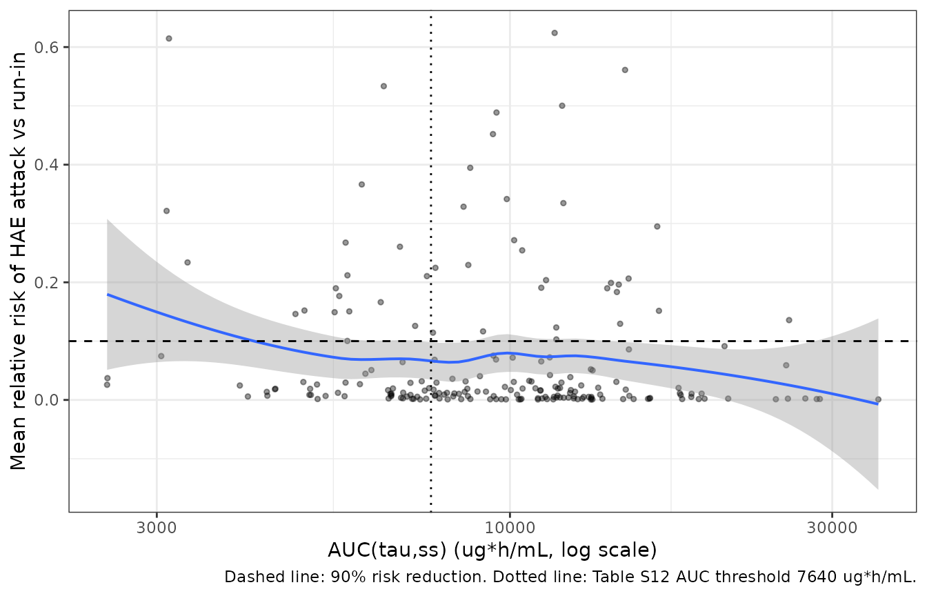
Replicates Figure 5 of Garcia 2025: relative risk of HAE attack versus steady-state exposure.
# Population-mean relative risk at steady state; Table S11 total row = 0.0835.
stopifnot(abs(mean(er_sub$rrbar) - 0.0835) < 0.04)
The population-mean relative risk at steady state is 0.0724, against the Table S11 total-row value of 0.0835. Note that the mean relative risk is far higher than the typical-value relative risk at the same exposure, because the interindividual variance on the hazard EC50 is very large (variance 4.95, CV% 1180): individuals in the upper tail of EC50 retain substantial attack risk and dominate the population mean. This is why the source defines its therapeutic thresholds on population-mean predictions rather than on the typical-value trajectory.
Assumptions and deviations
Errata found in the source
-
Table S7 covariance row labels are swapped. As
printed, the final-model row
gamma-E0 = 0.0846implies a correlation of0.0846 / sqrt(0.150 * 0.0268) = 1.334, which is mathematically impossible. The table’s own correlation column identifies the correct pairing in both the base-model and final-model columns:0.0846 / sqrt(0.150 * 0.168) = 0.533is the printedgamma-E0correlation, and0.0254 / sqrt(0.150 * 0.0268) = 0.401is the printedgamma-E50correlation (base model: 0.462 and 0.397 respectively). The value printed againstgamma-E0is thereforecov(gamma, EC50)and the value printed againstgamma-E50iscov(gamma, E0). The corrected assignment is used in the model file and yields a positive-definite matrix; the uncorrected reading does not. The same round-trip applied to the PK block (Table S5) reproduces all three printed correlations with the labels as printed, so the swap is specific to Table S7. -
kaunit label. Table S4 labels the absorption rate constant “(L/h)”;kais a first-order rate constant with units 1/h. -
Table 1 half-life footnote. Footnote
brenderst1/2 = 445 has “8.5 days”; 445 h is 18.5 days. Footnotea(tmax139 h = “5.8 days”) is correct, so a leading digit appears to have been dropped.
Parameters not reported in any available source
-
Baseline FXIIa-mediated kallikrein activity on
E0andEC50. This covariate was retained in the source’s final PopPK/PD model (Methods S1:LE0PD = THETA(5)*LOG(BLPD2/0.134),LEC50PD = THETA(6)*LOG(BLPD2/0.134)), but neither coefficient is reported: Table S6 tabulates only the four structural PD parameters, and the only rendering is the Figure S6 forest plot (EC50 only, no E0 panel), an image with no data table whose x-axis anchors – the 10th and 90th percentiles of baseline kallikrein activity – are not tabulated in any available source. The coefficients are therefore not digitisable. The packaged PD model is accordingly the reference-subject model at baseline kallikrein activity 0.134 POB, where both covariate terms are exactly zero by construction and the Table S6 structural estimates apply directly. The source’s own conclusion is that this covariate is not clinically meaningful. Recorded in the model file’scovariatesDataExcluded. -
ER covariate coefficients. Age, sex, prior HAE
treatment, and the HAE-FXII subtype are estimated on both the baseline
hazard and the hazard EC50 in the Methods S2 control stream, but Table
S8 tabulates only the five structural ER parameters and Figure 3 renders
conditional attack-rate predictions rather than coefficients. The
packaged ER model is therefore the reference-subject model defined by
Table S10 and the Figure 3 caption: 41 years of age, female, non-Chinese
and non-Japanese, HAE-C1INH-Type1/2, and no prior HAE treatment.
Baseline body weight and the baseline attack rate were screened but held
at
0 FIX, and all sixteen concomitant/rescue-medication coefficients are0 FIX. All are recorded incovariatesDataExcluded.
Modelling choices
-
Sequential fit packaged as a single simulatable
model. The source fitted the PD and ER models with the
individual PK parameters fixed at the PopPK empirical Bayes estimates
(
CLI,V2I, … in the$INPUTrecords). The packaged models instead regenerate PK from the population PK model with its own IIV block, which is the standard forward-simulation form. A consequence is that the PK and PD (or PK and hazard) random effects are independent here; the source did not estimate cross-covariances between them, so no information is lost, but individual PK-PD alignment is not preserved subject by subject. -
Imaxin the ER model. Table S8 reports “1 (fixed)” and the main text says “a fixed Imax value of 1”, but the Methods S2 control stream implementsEMAX = 1/(1+EXP(-THETA(4)))withTHETA(4) = 7 FIX, i.e. 0.999089. The control-stream value is used, because an Imax of exactly 1 drives the hazard to exactly zero at high concentration. -
ON_TREATMENTcovariate. The source applies the placebo/study effect viaIF (TAFD .GT. 0). This is encoded as an explicit time-varyingON_TREATMENTcovariate rather than viarxode2::tafd()so that the untreated run-in period remains simulatable, which matters because the run-in hazard is the denominator of the relative risk the paper reports. -
Placeholder residual on the ER model. The source
fits the RTTE model with an event-density likelihood
(
Y = 2*LAMBDA - 2*DV*LOG(LAMBDA)), so there is no observation-error model to translate. A negligible additive residual (addSd = 0.001) is attached to the survivor-function output so the nlmixr2 likelihood machinery accepts the model for forward simulation. -
Numerical guard.
max(Cc, 0)is applied before raising concentration to the non-integer Hill exponent, so a transiently negative solver value cannot produceNaN. This is a no-op for physically meaningful states. - Virtual cohort covariates. Body weight is drawn log-normally to match the reported median and truncated to the reported range; the paper’s own NHANES-based adolescent sampling is not reproducible from the available sources. All other covariates are held at the reference-subject values.
-
Dosing interval. A 30-day interval is simulated
throughout (the phase III regimen). Table 1’s
n = 173column pools phase II (28-day) and phase III (30-day) data.