Fosfomycin (Edwina 2023)
Source:vignettes/articles/Edwina_2023_fosfomycin.Rmd
Edwina_2023_fosfomycin.RmdModel and source
Edwina et al. (2023) re-analysed a crossover study in eight healthy men who received intravenous fosfomycin both as intermittent infusions (8 g over 30 min every 8 h, three doses) and as a continuous infusion (an 8 g 30-min loading dose followed by 1 g/h for 18 h). Plasma and urine concentrations were fitted together in NONMEM. The final model has two compartments plus a urine compartment. All elimination is renal, and the renal clearance scales with the CKD-EPI estimated GFR in absolute mL/min. The paper then used Monte Carlo simulation to compute the probability of target attainment (PTA) for Escherichia coli across a range of regimens.
- Citation: Edwina AE, Koch BCP, Muller AE, al Jalali V, Matzneller P, Zeitlinger M, Sassen SDT. Population plasma and urine pharmacokinetics and the probability of target attainment of fosfomycin in healthy male volunteers. Eur J Clin Pharmacol. 2023;79(6):775.
- Article: https://doi.org/10.1007/s00228-023-03477-5
- The final NONMEM control stream is in Supplementary file 3 and fixes the covariate form, the reference eGFR and the residual-error coding used below.
mod <- rxode2::rxode2(readModelDb("Edwina_2023_fosfomycin"))
#> ℹ parameter labels from comments will be replaced by 'label()'
mod_typ <- rxode2::zeroRe(mod)
Population
Eight healthy male volunteers (Table 1) aged 23-42 years (median 36.5), weighing 53-93 kg (median 83.5), with normal serum albumin and total protein. CKD-EPI eGFR ranged from 89 to 138 mL/min (median 119.63). Cockcroft-Gault creatinine clearance ranged from 97 to 151 mL/min. There were 176 plasma and 86 urine samples. Urine was collected over 0-3, 3-8, 8-16, 16-18, 18-20, 20-22 and 22-24 h for the intermittent regimen and up to 18 h for the continuous regimen.
The individual eGFR values used below were digitised by the maintainers from Supplementary Figure S2 (individual clearance against eGFR). Their range, 89-138 mL/min, matches Table 1.
study_egfr <- c(89, 109, 111, 115, 126, 132, 137, 138)
c(median = median(study_egfr), min = min(study_egfr), max = max(study_egfr))
#> median    min    max
#>  120.5   89.0  138.0
readModelDb("Edwina_2023_fosfomycin")$populationSource trace
| Equation / parameter | Value | Source location |
|---|---|---|
| Two-compartment model with a urine compartment; IV infusion into central | – | Figure 1; Supplementary file 3 $MODEL,
$DES
|
CL = CLpop * (eGFR/120)^beta * exp(eta); CL is the only
elimination route (K13 = CLR/V1) |
– | Table 2; Supplementary file 3 $PK
|
| eGFR is the CKD-EPI estimate in absolute mL/min (not BSA-normalised) | – | Methods (covariate analysis); Supplementary Table 4 models 11 vs 12 |
| Urine prediction = urine amount / collected urine volume | – | Supplementary file 3 S3 = UVL,
UVL = UVOL
|
Proportional error for plasma and urine,
W = IPRED * THETA, SIGMA 1 FIX
|
– | Results; Supplementary file 3 $ERROR,
$SIGMA
|
lcl (CLpop) |
6.34 L/h | Table 2 |
e_crcl_cl (beta) |
0.774 | Table 2 |
lq (Q) |
11.8 L/h | Table 2 |
lvc (Vc) |
10.2 L | Table 2 |
lvp (Vp) |
9.74 L | Table 2 |
etalcl (IIV CL) |
4.8 %CV -> omega^2 = log(0.048^2 + 1) | Table 2 |
propSd (plasma) |
38.17 % | Table 2 |
propSd_Curine (urine) |
87.15 % | Table 2 |
Regimens and simulation helpers
The PTA simulations in the paper cover five intermittent regimens (30-min infusions) and three continuous-infusion rates. Each continuous regimen is an 8 g 30-min loading dose followed by the stated rate for 18 h, as in the clinical study. This reading is confirmed below: the continuous-infusion AUCs in Figure 7 are reproduced only when the 18-hour infusion follows the loading dose.
regimens <- tibble::tribble(
  ~regimen,   ~type, ~amt, ~tau, ~rate_ci,
  "4 g/12 h", "II",  4000, 12,   NA,
  "4 g/8 h",  "II",  4000, 8,    NA,
  "4 g/6 h",  "II",  4000, 6,    NA,
  "8 g/12 h", "II",  8000, 12,   NA,
  "8 g/8 h",  "II",  8000, 8,    NA,
  "0.5 g/h",  "CI",  NA,   NA,   500,
  "0.75 g/h", "CI",  NA,   NA,   750,
  "1 g/h",    "CI",  NA,   NA,   1000
) |>
  dplyr::mutate(regimen = factor(regimen, levels = regimen))

dose_table <- function(reg_row) {
  if (reg_row$type == "II") {
    tibble::tibble(
      time = seq(0, 24 - 1e-6, by = reg_row$tau),
      amt = reg_row$amt,
      rate = reg_row$amt / 0.5
    )
  } else {
    tibble::tibble(
      time = c(0, 0.5),
      amt = c(8000, reg_row$rate_ci * 18),
      rate = c(8000 / 0.5, reg_row$rate_ci)
    )
  }
}

obs_grid <- seq(0, 24, by = 0.02)

build_events <- function(subjects) {
  dplyr::bind_rows(lapply(seq_len(nrow(subjects)), function(i) {
    s <- subjects[i, ]
    reg_row <- regimens[regimens$regimen == s$regimen, ]
    dplyr::bind_rows(
      dose_table(reg_row) |> dplyr::mutate(evid = 1L, cmt = "central"),
      tibble::tibble(time = obs_grid, evid = 0L, cmt = "central", dvid = 1L)
    ) |>
      dplyr::mutate(id = s$id, CRCL = s$CRCL, URINE_VOL_INTERVAL = 1000)
  })) |>
    dplyr::arrange(id, time, dplyr::desc(evid))
}

trapz <- function(t, y) sum(diff(t) * (head(y, -1) + tail(y, -1)) / 2)

# Deterministic solves on the zero-variability model. rxode2 warns that a
# multi-subject solve has no omega, which is intended here.
solve_typ <- function(events, ...) {
  suppressWarnings(rxode2::rxSolve(
    mod_typ,
    events = events, returnType = "data.frame",
    atol = 1e-9, rtol = 1e-9, ...
  ))
}
Typical exposure by eGFR (Figure 7)
Figure 7 shows the simulated plasma AUC24h/MIC for MIC 32 mg/L at eGFR 90, 110, 120 and 140 mL/min after 8 g every 8 h and after 1 g/h continuous infusion. The medians below were digitised by the maintainers from that figure. The typical-value solves use eta = 0, which is the median of a log-normal clearance.
typ_subj <- tidyr::expand_grid(
  regimen = factor(c("8 g/8 h", "1 g/h"), levels = levels(regimens$regimen)),
  CRCL = c(90, 110, 120, 140)
) |>
  dplyr::mutate(id = dplyr::row_number())

sim_typ <- solve_typ(build_events(typ_subj))
#> ℹ omega/sigma items treated as zero: 'etalcl'

fig7 <- sim_typ |>
  dplyr::group_by(id) |>
  dplyr::summarise(auc24 = trapz(time, Cc), .groups = "drop") |>
  dplyr::left_join(typ_subj, by = "id") |>
  dplyr::mutate(
    auc_mic32 = auc24 / 32,
    digitised = c(139, 121, 114, 102, 153, 133, 125, 112)[
      match(paste(regimen, CRCL), paste(
        rep(c("8 g/8 h", "1 g/h"), each = 4), rep(c(90, 110, 120, 140), 2)
      ))
    ],
    pct_diff = 100 * (auc_mic32 / digitised - 1)
  )

fig7 |>
  dplyr::select(regimen, CRCL, auc24, auc_mic32, digitised, pct_diff) |>
  dplyr::rename(
    "Regimen" = regimen, "eGFR (mL/min)" = CRCL, "AUC0-24 (mg h/L)" = auc24,
    "AUC24/MIC 32 (model)" = auc_mic32, "Figure 7 median (digitised)" = digitised,
    "% difference" = pct_diff
  ) |>
knitr::kable(digits = 1)| Regimen | eGFR (mL/min) | AUC0-24 (mg h/L) | AUC24/MIC 32 (model) | Figure 7 median (digitised) | % difference |
|---|---|---|---|---|---|
| 8 g/8 h | 90 | 4446.7 | 139.0 | 139 | 0.0 |
| 8 g/8 h | 110 | 3873.9 | 121.1 | 121 | 0.0 |
| 8 g/8 h | 120 | 3644.2 | 113.9 | 114 | -0.1 |
| 8 g/8 h | 140 | 3264.6 | 102.0 | 102 | 0.0 |
| 1 g/h | 90 | 4903.2 | 153.2 | 153 | 0.1 |
| 1 g/h | 110 | 4253.1 | 132.9 | 133 | -0.1 |
| 1 g/h | 120 | 3994.2 | 124.8 | 125 | -0.1 |
| 1 g/h | 140 | 3568.7 | 111.5 | 112 | -0.4 |
# Typical-value solves against values read off a figure: the reading error
# is about 1-2 units on a 100-160 axis.
stopifnot(max(abs(fig7$pct_diff)) < 3)
The model reproduces every Figure 7 median to within the reading accuracy of the plot. Because these values sit on the eGFR effect, they confirm both the exponent of 0.774 and the reference value of 120 mL/min.
Time above MIC (Figure 5)
Figure 5 shows %T>MIC over 24 h at MIC 32 mg/L for every simulated regimen. The medians below were digitised by the maintainers. The typical subject has eGFR 120 mL/min.
tmic_subj <- tibble::tibble(regimen = regimens$regimen, CRCL = 120) |>
  dplyr::mutate(id = dplyr::row_number())

sim_tmic <- solve_typ(build_events(tmic_subj))
#> ℹ omega/sigma items treated as zero: 'etalcl'

fig5 <- sim_tmic |>
  dplyr::group_by(id) |>
  dplyr::summarise(tmic32 = 100 * mean(Cc[time > 0] > 32), .groups = "drop") |>
  dplyr::left_join(tmic_subj, by = "id") |>
  dplyr::mutate(
    digitised = c(48.5, 75.5, 98.5, 69.5, 100, 88, 94.5, 98.5),
    diff_pts = tmic32 - digitised
  )

fig5 |>
  dplyr::select(regimen, tmic32, digitised, diff_pts) |>
  dplyr::rename(
    "Regimen" = regimen, "%T>MIC 32 (model)" = tmic32,
    "Figure 5 median (digitised)" = digitised, "Difference (points)" = diff_pts
  ) |>
knitr::kable(digits = 1)| Regimen | %T>MIC 32 (model) | Figure 5 median (digitised) | Difference (points) |
|---|---|---|---|
| 4 g/12 h | 48.8 | 48.5 | 0.2 |
| 4 g/8 h | 75.8 | 75.5 | 0.2 |
| 4 g/6 h | 99.1 | 98.5 | 0.6 |
| 8 g/12 h | 69.8 | 69.5 | 0.2 |
| 8 g/8 h | 99.9 | 100.0 | -0.1 |
| 0.5 g/h | 88.5 | 88.0 | 0.5 |
| 0.75 g/h | 94.5 | 94.5 | 0.0 |
| 1 g/h | 98.8 | 98.5 | 0.2 |
Probability of target attainment (Supplementary Tables 1 and 2)
The model has inter-individual variability only on clearance. AUC0-24
and %T>MIC therefore both decrease monotonically in the clearance
eta. A subject attains a target exactly when their eta lies below a
threshold, so the PTA is pnorm(eta* / omega), where eta* is
the eta at which the metric equals the target. The calculation below
solves a grid of etas from -5 to +5 omega, interpolates eta* and
evaluates the normal CDF. No random sampling is involved, so the result
does not depend on a seed.
omega <- sqrt(est[["etalcl"]])
eta_grid <- seq(-5, 5, by = 0.25) * omega

pta_subj <- dplyr::bind_rows(
  tidyr::crossing(regimen = regimens$regimen, CRCL = 120),
  tidyr::expand_grid(
    regimen = factor(c("8 g/8 h", "1 g/h"), levels = levels(regimens$regimen)),
    CRCL = c(90, 110, 140)
  )
) |>
  tidyr::crossing(eta = eta_grid) |>
  dplyr::mutate(id = dplyr::row_number())

# Each subject carries its own clearance: log CL shifted by its grid eta.
sim_pta <- solve_typ(
  build_events(pta_subj),
  params = data.frame(id = pta_subj$id, lcl = est[["lcl"]] + pta_subj$eta)
)
#> ℹ omega/sigma items treated as zero: 'etalcl'

mic_grid <- c(4, 8, 16, 32, 64, 128)
metrics <- sim_pta |>
  dplyr::group_by(id) |>
  dplyr::summarise(
    auc24 = trapz(time, Cc),
    tmic = list(vapply(mic_grid, function(m) 100 * mean(Cc[time > 0] > m), numeric(1))),
    .groups = "drop"
  ) |>
  dplyr::left_join(pta_subj, by = "id")

# PTA from a metric that decreases in eta: P(eta < eta*) with
# metric(eta*) = target.
pta_from_grid <- function(metric, eta, target) {
  y <- metric - target
  if (all(y >= 0)) return(100)
  if (all(y < 0)) return(0)
  keep <- !duplicated(y)
  100 * stats::pnorm(stats::approx(y[keep], eta[keep], xout = 0)$y / omega)
}

pta <- metrics |>
  dplyr::arrange(regimen, CRCL, eta) |>
  dplyr::group_by(regimen, CRCL) |>
  dplyr::group_modify(function(d, key) {
    tibble::tibble(
      MIC = mic_grid,
      auc989 = vapply(mic_grid, function(m) pta_from_grid(log(d$auc24 / m), d$eta, log(98.9)), numeric(1)),
      auc83 = vapply(mic_grid, function(m) pta_from_grid(log(d$auc24 / m), d$eta, log(83)), numeric(1)),
      auc25 = vapply(mic_grid, function(m) pta_from_grid(log(d$auc24 / m), d$eta, log(25)), numeric(1)),
      tmic75 = vapply(seq_along(mic_grid), function(j) {
        pta_from_grid(vapply(d$tmic, `[`, numeric(1), j), d$eta, 75)
      }, numeric(1))
    )
  }) |>
  dplyr::ungroup()
Which AUC target?
The Abstract and Methods state a bactericidal plasma target of AUC24h/MIC 83. The headers of Supplementary Tables 1 and 2, and the target lines drawn in Figures 7 and 8, use 98.9. The 0.5 g/h continuous infusion at MIC 32 mg/L decides between them: the paper reports 0% PTA, the 98.9 target gives 0%, and the 83 target would give about 40%.
pta |>
  dplyr::filter(CRCL == 120, MIC == 32, regimen %in% c("0.5 g/h", "0.75 g/h", "8 g/12 h")) |>
  dplyr::mutate(published = c(0, 0, 82.8)[match(regimen, c("8 g/12 h", "0.5 g/h", "0.75 g/h"))]) |>
  dplyr::select(regimen, published, auc989, auc83) |>
  dplyr::rename(
    "Regimen (MIC 32)" = regimen, "Supplementary Table 1 (%)" = published,
    "Model, target 98.9 (%)" = auc989, "Model, target 83 (%)" = auc83
  ) |>
knitr::kable(digits = 1)| Regimen (MIC 32) | Supplementary Table 1 (%) | Model, target 98.9 (%) | Model, target 83 (%) |
|---|---|---|---|
| 8 g/12 h | 0.0 | 0 | 6.5 |
| 0.5 g/h | 0.0 | 0 | 40.6 |
| 0.75 g/h | 82.8 | 84 | 100.0 |
The PTA comparison below therefore uses 98.9.
Comparison with the supplementary tables
Supplementary Table 1 (eGFR 120 mL/min, all regimens) and Supplementary Table 2 (eGFR 90-140 mL/min, 8 g every 8 h and 1 g/h) are transcribed below. They are compared only for MIC 4-128 mg/L, because every regimen reaches 100% below MIC 4 and 0% above MIC 128.
mics <- mic_grid
tab1 <- tibble::tribble(
  ~regimen,   ~auc989,                       ~auc25,                       ~tmic75,
  "4 g/12 h", c(100, 100, 0, 0, 0, 0),       c(100, 100, 100, 100, 0, 0),  c(98.6, 6.9, 6.9, 0, 0, 0),
  "4 g/8 h",  c(100, 100, 99.8, 0, 0, 0),    c(100, 100, 100, 100, 99.6, 0), c(100, 100, 100, 54.7, 0, 0),
  "4 g/6 h",  c(100, 100, 99.4, 0, 0, 0),    c(100, 100, 100, 100, 98.3, 0), c(100, 100, 100, 100, 0.1, 0),
  "8 g/12 h", c(100, 100, 100, 0, 0, 0),     c(100, 100, 100, 100, 100, 0), c(100, 99.9, 99.9, 6.9, 0, 0),
  "8 g/8 h",  c(100, 100, 100, 99.8, 0, 0),  c(100, 100, 100, 100, 100, 99.6), c(100, 100, 100, 100, 54.7, 0),
  "0.5 g/h",  c(100, 100, 100, 0, 0, 0),     c(100, 100, 100, 100, 100, 0), c(100, 100, 100, 100, 100, 0),
  "0.75 g/h", c(100, 100, 100, 82.8, 0, 0),  c(100, 100, 100, 100, 100, 76.7), c(100, 100, 100, 100, 100, 8.3),
  "1 g/h",    c(100, 100, 100, 100, 0, 0),   c(100, 100, 100, 100, 100, 100), c(100, 100, 100, 100, 100, 100)
) |>
  dplyr::mutate(CRCL = 120)
tab2 <- tibble::tribble(
  ~regimen,  ~CRCL, ~auc989,                       ~auc25,                          ~tmic75,
  "1 g/h",   90,    c(100, 100, 100, 100, 0, 0),   c(100, 100, 100, 100, 100, 100), c(100, 100, 100, 100, 100, 100),
  "1 g/h",   110,   c(100, 100, 100, 100, 0, 0),   c(100, 100, 100, 100, 100, 100), c(100, 100, 100, 100, 100, 100),
  "1 g/h",   140,   c(100, 100, 100, 99.6, 0, 0),  c(100, 100, 100, 100, 100, 98.8), c(100, 100, 100, 100, 100, 97.4),
  "8 g/8 h", 90,    c(100, 100, 100, 100, 0, 0),   c(100, 100, 100, 100, 100, 100), c(100, 100, 100, 100, 100, 0),
  "8 g/8 h", 110,   c(100, 100, 100, 100, 0, 0),   c(100, 100, 100, 100, 100, 100), c(100, 100, 100, 100, 93.7, 0),
  "8 g/8 h", 140,   c(100, 100, 100, 74.2, 0, 0),  c(100, 100, 100, 100, 100, 68.1), c(100, 100, 100, 100, 0.7, 0)
)
published <- dplyr::bind_rows(tab1, tab2) |>
  dplyr::mutate(MIC = list(mics)) |>
  tidyr::unnest(c(MIC, auc989, auc25, tmic75)) |>
  tidyr::pivot_longer(c(auc989, auc25, tmic75), names_to = "target", values_to = "published") |>
  dplyr::mutate(regimen = factor(regimen, levels = levels(regimens$regimen)))

pta_cmp <- pta |>
  dplyr::select(-auc83) |>
  tidyr::pivot_longer(c(auc989, auc25, tmic75), names_to = "target", values_to = "model") |>
  dplyr::inner_join(published, by = c("regimen", "CRCL", "MIC", "target")) |>
  dplyr::mutate(
    target = dplyr::recode(target, auc989 = "AUC24/MIC 98.9", auc25 = "AUC24/MIC 25", tmic75 = "75%T>MIC"),
    diff_pts = model - published
  )

pta_cmp |>
  dplyr::filter(published > 0 & published < 100 | (model > 0.5 & model < 99.5)) |>
  dplyr::arrange(target, regimen, CRCL, MIC) |>
  dplyr::rename(
    "Target" = target, "Regimen" = regimen, "eGFR (mL/min)" = CRCL, "MIC (mg/L)" = MIC,
    "Model PTA (%)" = model, "Published PTA (%)" = published, "Difference (points)" = diff_pts
  ) |>
knitr::kable(digits = 1, caption = "Cells where either the model or the paper is between 0% and 100%.")| Regimen | eGFR (mL/min) | MIC (mg/L) | Target | Model PTA (%) | Published PTA (%) | Difference (points) |
|---|---|---|---|---|---|---|
| 4 g/12 h | 120 | 4 | 75%T>MIC | 100.0 | 98.6 | 1.4 |
| 4 g/12 h | 120 | 8 | 75%T>MIC | 100.0 | 6.9 | 93.1 |
| 4 g/12 h | 120 | 16 | 75%T>MIC | 6.4 | 6.9 | -0.5 |
| 4 g/8 h | 120 | 32 | 75%T>MIC | 57.4 | 54.7 | 2.7 |
| 4 g/6 h | 120 | 64 | 75%T>MIC | 0.4 | 0.1 | 0.3 |
| 8 g/12 h | 120 | 8 | 75%T>MIC | 100.0 | 99.9 | 0.1 |
| 8 g/12 h | 120 | 16 | 75%T>MIC | 100.0 | 99.9 | 0.1 |
| 8 g/12 h | 120 | 32 | 75%T>MIC | 6.4 | 6.9 | -0.5 |
| 8 g/8 h | 110 | 64 | 75%T>MIC | 94.8 | 93.7 | 1.1 |
| 8 g/8 h | 120 | 64 | 75%T>MIC | 57.4 | 54.7 | 2.7 |
| 8 g/8 h | 140 | 64 | 75%T>MIC | 1.2 | 0.7 | 0.5 |
| 0.75 g/h | 120 | 128 | 75%T>MIC | 7.5 | 8.3 | -0.8 |
| 1 g/h | 140 | 128 | 75%T>MIC | 96.4 | 97.4 | -1.0 |
| 4 g/8 h | 120 | 64 | AUC24/MIC 25 | 99.8 | 99.6 | 0.2 |
| 4 g/6 h | 120 | 64 | AUC24/MIC 25 | 100.0 | 98.3 | 1.7 |
| 8 g/8 h | 120 | 128 | AUC24/MIC 25 | 99.8 | 99.6 | 0.2 |
| 8 g/8 h | 140 | 128 | AUC24/MIC 25 | 67.3 | 68.1 | -0.8 |
| 0.75 g/h | 120 | 128 | AUC24/MIC 25 | 77.4 | 76.7 | 0.7 |
| 1 g/h | 140 | 128 | AUC24/MIC 25 | 99.1 | 98.8 | 0.3 |
| 4 g/8 h | 120 | 16 | AUC24/MIC 98.9 | 99.9 | 99.8 | 0.1 |
| 4 g/6 h | 120 | 16 | AUC24/MIC 98.9 | 100.0 | 99.4 | 0.6 |
| 8 g/8 h | 120 | 32 | AUC24/MIC 98.9 | 99.9 | 99.8 | 0.1 |
| 8 g/8 h | 140 | 32 | AUC24/MIC 98.9 | 75.6 | 74.2 | 1.4 |
| 0.75 g/h | 120 | 32 | AUC24/MIC 98.9 | 84.0 | 82.8 | 1.2 |
| 1 g/h | 140 | 32 | AUC24/MIC 98.9 | 99.6 | 99.6 | 0.0 |
Every cell where either side lies strictly between 0% and 100% is reproduced to within 3 percentage points, with one exception:
- 4 g every 12 h, 75%T>MIC at MIC 8 mg/L. The paper gives 6.9%, the same value as its MIC 16 row; the model gives 100%. In a linear model, doubling the dose has the same effect as halving the MIC, so 4 g every 12 h at MIC 8 must equal 8 g every 12 h at MIC 16, for which the paper itself reports 99.9%. The published 6.9% looks like the MIC 16 row repeated, and the cell is excluded from the check below.
One further pattern in Supplementary Table 1 is internally inconsistent, although the model is within 2 points of each cell. The paper reports lower AUC-based PTAs for 4 g every 6 h than for 4 g every 8 h (99.4% vs 99.8% at MIC 16 for the 98.9 target, and 98.3% vs 99.6% at MIC 64 for the 25 target). A regimen that gives 16 g/day cannot have a lower AUC0-24 than one that gives 12 g/day. The model gives AUC0-24 of 2390 mg h/L for 4 g every 6 h, against 1820 mg h/L for 4 g every 8 h. The near-100% PTAs are not sensitive enough to show the difference.
pta_checked <- pta_cmp |>
  dplyr::filter(!(regimen == "4 g/12 h" & target == "75%T>MIC" & MIC == 8))
c(cells = nrow(pta_checked), max_abs_diff = max(abs(pta_checked$diff_pts)))
#>        cells max_abs_diff
#>   251.000000     2.736569

# The model side is an exact normal CDF; the paper's side carries the Monte
# Carlo error of 1000 subjects, about 1.3 points at 80% PTA.
stopifnot(max(abs(pta_checked$diff_pts)) < 5)
Stochastic simulation of the clinical study
The eight study subjects (digitised eGFR values, above) are replicated 25 times per regimen, giving 200 virtual subjects per arm. Each receives the study’s intermittent regimen (8 g every 8 h, three doses) and its continuous regimen (8 g loading dose + 1 g/h for 18 h).
rxode2::rxSetSeed(2023)
n_rep <- 25
study_subj <- tidyr::expand_grid(
  regimen = factor(c("8 g/8 h", "1 g/h"), levels = levels(regimens$regimen)),
  rep = seq_len(n_rep),
  CRCL = study_egfr
) |>
  dplyr::mutate(id = dplyr::row_number())

study_events <- build_events(study_subj) |>
  dplyr::filter(evid == 1L | abs(time * 4 - round(time * 4)) < 1e-9)

sim_study <- rxode2::rxSolve(
  mod,
  events = study_events, returnType = "data.frame"
) |>
  dplyr::left_join(dplyr::select(study_subj, id, regimen), by = "id")
Supplementary Figure S1 shows the observed mean plasma concentrations and cumulative urinary excretion for each regimen. The means below were digitised by the maintainers from that figure.
obs_plasma <- dplyr::bind_rows(
  tibble::tibble(
    regimen = "8 g/8 h",
    time = c(0.5, 8, 8.5, 16, 16.5, 17, 17.5, 18, 20, 21, 22, 24),
    Cc = c(520, 29, 560, 46, 540, 320, 265, 225, 108, 85, 65, 39)
  ),
  tibble::tibble(
    regimen = "1 g/h",
    time = c(0.5, 1, 3, 5, 8, 16, 17, 18),
    Cc = c(570, 320, 235, 207, 185, 182, 186, 185)
  )
) |>
  dplyr::mutate(regimen = factor(regimen, levels = levels(regimens$regimen)))
vpc <- sim_study |>
  dplyr::group_by(regimen, time) |>
  dplyr::summarise(
    med = median(Cc), lo = quantile(Cc, 0.05), hi = quantile(Cc, 0.95),
    .groups = "drop"
  )

ggplot(vpc[vpc$time > 0, ], aes(time, med)) +
  geom_ribbon(aes(ymin = lo, ymax = hi), alpha = 0.25) +
  geom_line() +
  geom_point(data = obs_plasma, aes(time, Cc), colour = "red") +
  facet_wrap(~regimen) +
  scale_y_log10() +
  labs(x = "Time after first dose (h)", y = "Fosfomycin plasma (mg/L)")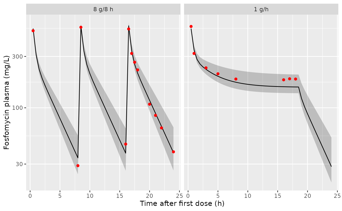
Simulated plasma fosfomycin (median and 90% prediction interval of the individual predictions, 200 subjects per regimen) with the observed means digitised from Supplementary Figure S1 (points). Compare with Figure 3A of Edwina 2023.
obs_vs_sim <- obs_plasma |>
  dplyr::left_join(vpc, by = c("regimen", "time")) |>
  dplyr::mutate(ratio = med / Cc)
obs_vs_sim |>
  dplyr::select(regimen, time, Cc, med, ratio) |>
  dplyr::rename(
    "Regimen" = regimen, "Time (h)" = time, "Observed mean (digitised, mg/L)" = Cc,
    "Simulated median (mg/L)" = med, "Ratio" = ratio
  ) |>
knitr::kable(digits = 2)| Regimen | Time (h) | Observed mean (digitised, mg/L) | Simulated median (mg/L) | Ratio |
|---|---|---|---|---|
| 8 g/8 h | 0.5 | 520 | 544.80 | 1.05 |
| 8 g/8 h | 8.0 | 29 | 34.25 | 1.18 |
| 8 g/8 h | 8.5 | 560 | 574.58 | 1.03 |
| 8 g/8 h | 16.0 | 46 | 37.90 | 0.82 |
| 8 g/8 h | 16.5 | 540 | 577.75 | 1.07 |
| 8 g/8 h | 17.0 | 320 | 340.04 | 1.06 |
| 8 g/8 h | 17.5 | 265 | 253.89 | 0.96 |
| 8 g/8 h | 18.0 | 225 | 209.99 | 0.93 |
| 8 g/8 h | 20.0 | 108 | 117.38 | 1.09 |
| 8 g/8 h | 21.0 | 85 | 88.70 | 1.04 |
| 8 g/8 h | 22.0 | 65 | 67.03 | 1.03 |
| 8 g/8 h | 24.0 | 39 | 38.28 | 0.98 |
| 1 g/h | 0.5 | 570 | 544.32 | 0.95 |
| 1 g/h | 1.0 | 320 | 344.58 | 1.08 |
| 1 g/h | 3.0 | 235 | 227.74 | 0.97 |
| 1 g/h | 5.0 | 207 | 196.30 | 0.95 |
| 1 g/h | 8.0 | 185 | 172.80 | 0.93 |
| 1 g/h | 16.0 | 182 | 156.97 | 0.86 |
| 1 g/h | 17.0 | 186 | 156.51 | 0.84 |
| 1 g/h | 18.0 | 185 | 156.16 | 0.84 |
# Centre and robust spread only (see the package notes on cohort extremes):
# a mis-transcribed volume or clearance shifts every ratio by tens of percent.
stopifnot(
  abs(log(median(obs_vs_sim$ratio))) < log(1.15),
  quantile(abs(log(obs_vs_sim$ratio)), 0.9) < log(1.35)
)
The simulated median follows the observed means of the intermittent regimen throughout. During the continuous-infusion plateau (16-18 h) it is about 15% below the observed means.
Cumulative urinary excretion
All elimination in the model goes to the urine compartment. The cumulative percentage of the administered dose excreted therefore approaches 100% as the body empties, and urine plus body content always equals the dose given so far. The observed points are the means digitised from Supplementary Figure S1. Before fitting, the authors truncated cumulative amounts above the administered dose to the dose.
typ_dose_total <- c("8 g/8 h" = 24000, "1 g/h" = 26000)
urine_typ <- sim_typ |>
  dplyr::left_join(dplyr::select(typ_subj, id, regimen), by = "id") |>
  dplyr::filter(CRCL == 120) |>
  dplyr::mutate(
    pct_dose = 100 * urine / typ_dose_total[as.character(regimen)],
    body = central + peripheral1
  )

obs_urine <- dplyr::bind_rows(
  tibble::tibble(regimen = "8 g/8 h", time = c(3, 8, 16, 18, 20, 22, 24), pct = c(19, 31, 60, 84, 95, 99, 102)),
  tibble::tibble(regimen = "1 g/h", time = c(3, 8, 16, 18), pct = c(21, 50, 84, 99))
) |>
  dplyr::mutate(regimen = factor(regimen, levels = levels(regimens$regimen)))

ggplot(urine_typ, aes(time, pct_dose)) +
  geom_line() +
  geom_point(data = obs_urine, aes(time, pct), colour = "red") +
  facet_wrap(~regimen) +
  labs(x = "Time after first dose (h)", y = "Cumulative urinary excretion (% of dose)")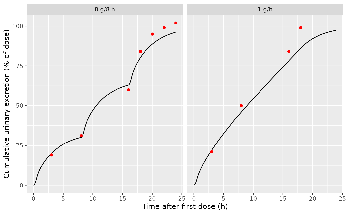
Typical cumulative urinary excretion (% of the total dose of each regimen; eGFR 120 mL/min) with the observed means digitised from Supplementary Figure S1 (points).
# Mass balance at 24 h: everything infused is in the urine or still in the
# body. Same parameters on both sides, so only solver error remains.
mb <- urine_typ |>
  dplyr::filter(time == 24) |>
  dplyr::mutate(total = urine + body, dose = typ_dose_total[as.character(regimen)])
stopifnot(max(abs(mb$total / mb$dose - 1)) < 1e-6)

obs_urine |>
  dplyr::left_join(dplyr::select(urine_typ, regimen, time, pct_dose), by = c("regimen", "time")) |>
  dplyr::mutate(diff_pts = pct_dose - pct) |>
  dplyr::rename(
    "Regimen" = regimen, "Time (h)" = time, "Observed mean (digitised, %)" = pct,
    "Model, typical (%)" = pct_dose, "Difference (points)" = diff_pts
  ) |>
knitr::kable(digits = 1)| Regimen | Time (h) | Observed mean (digitised, %) | Model, typical (%) | Difference (points) |
|---|---|---|---|---|
| 8 g/8 h | 3 | 19 | 20.0 | 1.0 |
| 8 g/8 h | 8 | 31 | 30.0 | -1.0 |
| 8 g/8 h | 16 | 60 | 63.0 | 3.0 |
| 8 g/8 h | 18 | 84 | 80.2 | -3.8 |
| 8 g/8 h | 20 | 95 | 88.7 | -6.3 |
| 8 g/8 h | 22 | 99 | 93.5 | -5.5 |
| 8 g/8 h | 24 | 102 | 96.3 | -5.7 |
| 1 g/h | 3 | 21 | 21.9 | 0.9 |
| 1 g/h | 8 | 50 | 45.9 | -4.1 |
| 1 g/h | 16 | 84 | 78.1 | -5.9 |
| 1 g/h | 18 | 99 | 85.9 | -13.1 |
The model excretes 96% (intermittent) and 97% (continuous) of the administered dose by 24 h. The paper reports that cumulative urinary excretion reached “around 100% of the daily dose”. For the intermittent regimen the model matches the observed means up to 16 h and runs 4-6 points below them afterwards, where the observed means reach or pass 100%. For the continuous regimen it runs 4-6 points below from 8 h and 13 points below at 18 h. The paper does not say whether the continuous-infusion percentages use the full 26 g or only the dose infused up to each collection, and the observed recovery exceeded the administered dose in six of eight subjects after intermittent and seven of eight after continuous infusion. The authors attribute this to urine-collection or assay error. The model cannot exceed 100% by construction.
Urine concentration per collection interval
A urinary observation is the amount excreted during one collection
interval divided by the volume collected
(Curine = urine / URINE_VOL_INTERVAL). In rxode2 the urine
state is emptied at each interval boundary with a replacement event
(evid = 5, amt = 0). The event is placed a
numerical epsilon after the boundary, so that the end-of-interval
observation is read first. The interval volumes below are illustrative,
a constant 300 mL/h, because the paper does not report the individual
volumes. For the same reason, Figure 6 (urinary PTA) and the urine AUCs
of Figure 8 cannot be reproduced: they depend on the urine volumes the
authors assumed.
bounds <- c(3, 8, 16, 18, 20, 22, 24)
vols_ml <- 300 * diff(c(0, bounds))
reset_eps <- 1e-6
vol_for <- function(t) vols_ml[pmax(1, findInterval(t, c(0, bounds), left.open = TRUE))]

ev_int <- dplyr::bind_rows(
  dose_table(regimens[regimens$regimen == "8 g/8 h", ]) |>
    dplyr::mutate(evid = 1L, cmt = "central"),
  tibble::tibble(time = head(bounds, -1) + reset_eps, amt = 0, evid = 5L, cmt = "urine"),
  tibble::tibble(time = c(0, bounds), evid = 0L, cmt = "urine", dvid = 2L)
) |>
  dplyr::mutate(id = 1L, CRCL = 120, URINE_VOL_INTERVAL = vol_for(time)) |>
  dplyr::arrange(time, dplyr::desc(evid))

sim_int <- rxode2::rxSolve(mod_typ, events = ev_int, returnType = "data.frame",
                           atol = 1e-10, rtol = 1e-10) |>
  dplyr::filter(time %in% bounds)
#> ℹ omega/sigma items treated as zero: 'etalcl'
cum <- urine_typ |>
  dplyr::filter(regimen == "8 g/8 h", time %in% c(0, bounds)) |>
  dplyr::arrange(time)

int_tab <- tibble::tibble(
  interval = paste0(c(0, head(bounds, -1)), "-", bounds, " h"),
  volume = vols_ml,
  amount = sim_int$urine,
  curine = sim_int$Curine,
  cum_diff = diff(cum$urine)
)
int_tab |>
  dplyr::rename(
    "Interval" = interval, "Urine volume (mL)" = volume, "Amount in interval (mg)" = amount,
    "Curine (mg/L)" = curine, "Cumulative-run difference (mg)" = cum_diff
  ) |>
knitr::kable(digits = 1)| Interval | Urine volume (mL) | Amount in interval (mg) | Curine (mg/L) | Cumulative-run difference (mg) |
|---|---|---|---|---|
| 0-3 h | 900 | 4795.1 | 5327.9 | 4795.1 |
| 3-8 h | 1500 | 2405.3 | 1603.6 | 2405.3 |
| 8-16 h | 2400 | 7913.3 | 3297.2 | 7913.3 |
| 16-18 h | 600 | 4137.5 | 6895.9 | 4137.5 |
| 18-20 h | 600 | 2029.4 | 3382.3 | 2029.4 |
| 20-22 h | 600 | 1158.7 | 1931.2 | 1158.7 |
| 22-24 h | 600 | 665.0 | 1108.3 | 665.0 |
NCA of the simulated study (PKNCA)
PKNCA is run on the stochastic simulation of the study regimens over
0-24 h. The only NCA-type values the paper reports are the individual
maximum concentrations during the continuous-infusion regimen
(Supplementary Table 3: 491.25, 552.03, 730.99, 577.98, 564.18, 508.23,
456.44 and 522.20 mg/L; mean 550.41, median 537.1). These are reached at
the end of the 8 g loading infusion. The comparison uses the median,
because ncaComparisonTable() summarises the simulated
subjects by their median.
conc_nca <- sim_study |>
  dplyr::filter(!is.na(Cc)) |>
  dplyr::select(id, regimen, time, Cc)
stopifnot(all(conc_nca |> dplyr::group_by(id) |> dplyr::summarise(t0 = min(time)) |> dplyr::pull(t0) == 0))

dose_nca <- study_events |>
  dplyr::filter(evid == 1L) |>
  dplyr::left_join(dplyr::select(study_subj, id, regimen), by = "id") |>
  dplyr::mutate(duration = amt / rate) |>
  dplyr::select(id, regimen, time, amt, duration)

conc_obj <- PKNCA::PKNCAconc(conc_nca, Cc ~ time | regimen + id, concu = "mg/L", timeu = "h")
dose_obj <- PKNCA::PKNCAdose(dose_nca, amt ~ time | regimen + id, doseu = "mg",
                             route = "intravascular", duration = "duration")
intervals <- data.frame(start = 0, end = 24, cmax = TRUE, tmax = TRUE, auclast = TRUE)
nca <- PKNCA::pk.nca(PKNCA::PKNCAdata(conc_obj, dose_obj, intervals = intervals))

summary(nca)
#>  Interval Start Interval End regimen   N AUClast (h*mg/L) Cmax (mg/L)
#>               0           24 8 g/8 h 200      3640 [10.9]  581 [3.25]
#>               0           24   1 g/h 200      4010 [10.9]  546 [1.50]
#>              Tmax (h)
#>     16.5 [16.5, 16.5]
#>  0.500 [0.500, 0.500]
#>
#> Caption: AUClast, Cmax: geometric mean and geometric coefficient of variation; Tmax: median and range; N: number of subjects
st3 <- c(491.25, 552.03, 730.99, 577.98, 564.18, 508.23, 456.44, 522.20)
reference <- data.frame(regimen = "1 g/h", cmax = median(st3))
nca_res <- as.data.frame(nca$result) |>
  dplyr::filter(regimen == "1 g/h")
cmp <- nlmixr2lib::ncaComparisonTable(
  simulated = nca_res,
  reference = reference,
  by = "regimen",
  params = "cmax",
  units = c(cmax = "mg/L"),
  tolerance_pct = 20
)
cmp |>
  dplyr::rename("Regimen" = regimen) |>
knitr::kable(caption = "Simulated continuous-infusion Cmax against the median of Supplementary Table 3.")| NCA parameter | Regimen | Reference | Simulated | % diff |
|---|---|---|---|---|
| Cmax (mg/L) | 1 g/h | 537 | 544 | +1.3% |
sim_cmax <- median(nca_res$PPORRES[nca_res$PPTESTCD == "cmax"])
stopifnot(abs(sim_cmax / median(st3) - 1) < 0.10)
The simulated median Cmax at the end of the loading dose agrees with the observed median. Cmax is determined almost entirely by the central volume, which has no inter-individual variability in the final model. The simulated spread of Cmax therefore comes only from the small clearance variability, and is narrower than the observed range of 456-731 mg/L.
Assumptions and deviations
- AUC target 98.9 rather than 83. The paper’s text gives a bactericidal plasma target of AUC24h/MIC 83. The tables and figures it presents use 98.9, and only 98.9 reproduces them (see “Which AUC target?”).
- Two inconsistent cells in Supplementary Table 1 (4 g every 6 h AUC rows; 4 g every 12 h 75%T>MIC at MIC 4 and 8) are documented above and excluded from the numeric check.
- Continuous-infusion PTA regimens. These are taken to be an 8 g 30-min loading dose followed by the stated rate for 18 h, as in the clinical study. The Figure 7 and Figure 5 values are reproduced under this assumption.
-
Urine volume units. The control stream divides the
urine amount by
UVOLwithout stating its units. The canonicalURINE_VOL_INTERVALis in mL and is converted to L in the model, so that urinary concentrations are in mg/L, the assay’s unit. The source does not say how the urine compartment was emptied between collections. Theevid = 5reset shown above is the rxode2 equivalent of observing and then resetting the output compartment. - IIV conversion. Table 2 reports the clearance IIV as 4.8 %CV. It is encoded as omega^2 = log(0.048^2 + 1) = 0.0023. At this magnitude the alternative omega^2 = 0.048^2 differs by less than 0.1%.
- Albumin and total protein units. Table 1 labels these g/dL, but the values (44 and 69.45) are g/L. Neither is in the final model.
- Digitised values. The study eGFR values (Supplementary Figure S2), the observed mean plasma concentrations and urinary excretion (Supplementary Figure S1), and the Figure 5 and Figure 7 medians were read off the published figures by the maintainers. The assertions use tolerances that allow for this reading error.