Fludarabine (Ivaturi 2017)
Source:vignettes/articles/Ivaturi_2017_fludarabine.Rmd
Ivaturi_2017_fludarabine.RmdModel and source
- Citation: Ivaturi V, Dvorak CC, Chan D, Liu T, Cowan MJ, Wahlstrom J, Stricherz M, Jennissen C, Orchard PJ, Tolar J, Pai SY, Huang L, Aweeka F, Long-Boyle J. Pharmacokinetics and Model-Based Dosing to Optimize Fludarabine Therapy in Pediatric Hematopoietic Cell Transplant Recipients. Biol Blood Marrow Transplant. 2017;23(10):1701-1713. doi:10.1016/j.bbmt.2017.06.021
- Description: Two-compartment population PK model for plasma f-ara-a (the circulating nucleoside of intravenous fludarabine phosphate) in children and young adults undergoing hematopoietic cell transplantation, with allometric weight scaling (reference 15 kg) and a linear creatinine-clearance effect on clearance, linked to an intracellular f-ara-ATP compartment in peripheral blood mononuclear cells whose uptake rate constant declines as a power of time after the first dose.
- Article: https://doi.org/10.1016/j.bbmt.2017.06.021 (NIH author manuscript PMC6108324)
- Supplement: Supplemental Figures S1 (observed concentrations) and S2 (prediction-corrected VPC), available from PMC6108324.
Fludarabine phosphate (f-ara-AMP) is given intravenously and is dephosphorylated in plasma to the nucleoside f-ara-a, which is what circulates and what this model describes in plasma. f-ara-a enters cells and is phosphorylated to the cytotoxic triphosphate f-ara-ATP. Ivaturi 2017 is the first published model of f-ara-ATP in clinical samples from children undergoing hematopoietic cell transplantation (HCT). It links a two-compartment plasma f-ara-a model to a peripheral-blood-mononuclear-cell (PBMC) f-ara-ATP compartment. Weight and creatinine clearance (CRCL) are the only covariates.
The model was later refined by Brooks 2022 (Pharmaceutics 14:2462), which replaced weight with fat-free mass, added a maturation function on clearance and kept the PBMC parameters of this model fixed.
Population
The study was a prospective multicenter PK study (NCT01316549, 2010-2015) at three US centers. It enrolled children who were to undergo allogeneic HCT, or autologous HCT with gene therapy, with fludarabine in the conditioning regimen. 140 subjects contributed 840 f-ara-a and 239 f-ara-ATP concentrations to the PK model. f-ara-ATP was collected only at the UCSF site (n = 66).
Table 1 describes the 133 subjects who also entered the PK-PD analysis:
- Age: median 5.0 years (range 0.2-17.9).
- Weight: median 15.7 kg (range 3-111).
- Sex: 46% female.
- BSA: median 0.68 m^2.
- CRCL: median 150 mL/min/1.73 m^2 (range 35-150), estimated by Schwartz in children and by Cockcroft-Gault with ideal body weight in young adults.
- Diagnosis: 44% hematologic malignancy, 14% primary immune deficiency, 16% inherited metabolic disorder, 16% bone marrow failure, 6% hemoglobinopathy and 4% epidermolysis bullosa.
- Fludarabine phosphate: 40 mg/m^2 in 41%, 12.5-35 mg/m^2 in 30%, and 0.9-1.33 mg/kg in 29%. It was infused over 30-60 min once daily for 3-5 days.
The same information is available from the model’s
population metadata:
pop <- rxode2::rxode(readModelDb("Ivaturi_2017_fludarabine"))$population
#> ℹ parameter labels from comments will be replaced by 'label()'
str(pop, max.level = 1)
#> List of 13
#>  $ species       : chr "human"
#>  $ n_subjects    : num 140
#>  $ n_studies     : num 1
#>  $ age_range     : chr "0.2-17.9 years"
#>  $ age_median    : chr "5.0 years"
#>  $ weight_range  : chr "3-111 kg"
#>  $ weight_median : chr "15.7 kg"
#>  $ sex_female_pct: num 46
#>  $ disease_state : chr "children undergoing allogeneic hematopoietic cell transplantation (or autologous HCT with gene therapy) with fl"| __truncated__
#>  $ renal_function: chr "creatinine clearance median 150 (range 35-150) mL/min/1.73 m^2; serum creatinine median 0.3 (0.14-1.89) mg/dL"
#>  $ dose_range    : chr "fludarabine phosphate 12.5-40 mg/m^2 or 0.9-1.33 mg/kg IV over 30-60 min once daily for 3-5 days"
#>  $ regions       : chr "United States (UCSF Benioff Children's Hospital, University of Minnesota Masonic Children's Hospital, Boston Ch"| __truncated__
#>  $ notes         : chr "Prospective multicenter study NCT01316549, 2010-2015. 140 subjects completed PK assessments and were used for P"| __truncated__
Source trace
Each ini() entry in
inst/modeldb/specificDrugs/Ivaturi_2017_fludarabine.R
carries a comment giving its source. The table below collects them.
Values come from the Final Model column of Table 2. The clearance
equation is printed in Results (‘PopPK Analysis’).
| Equation / parameter | Value | Source location |
|---|---|---|
lcl (CL at 15 kg, CRCL 100) |
3.1 L/h | Table 2 ‘Typical value for f-ara-a CL, L/h/15 kg’ (RSE 3.3%) |
e_crcl_cl (CRCLEFF) |
0.006 per mL/min/1.73 m^2 | Table 2 ‘Effect of creatinine clearance on f-ara-a CL’ (RSE 9.5%) |
lvc (Vc at 15 kg) |
13.4 L | Table 2 ‘Vc, L/kg’ (RSE 6.3%); read per 15 kg, see Assumptions |
lq (Q at 15 kg) |
2.2 L/h | Table 2 ‘Intercompartmental CL, L/h/kg’ (RSE 10.4%); read per 15 kg |
lvp (Vp at 15 kg) |
13.4 L | Table 2 ‘Vp, L/15’ (RSE 4.8%) |
lkmet_faraatp (Kin) |
0.005 (pmol/10^6 cells)/h per ng/mL | Table 2 ‘K in’ (RSE 15.4%) |
e_time_kmet_faraatp |
-0.41 | Table 2 ‘Time effect on kin’ (RSE 12.7%); functional form inferred, see below |
lkel_faraatp (Kout) |
0.09 1/h | Table 2 ‘K out’ (RSE 7.2%) |
etalcl, etalvc,
etalkmet_faraatp
|
31.7, 38.3, 81.9 (omega x 100) | Table 2 IIV rows; omega^2 = (P/100)^2, see Assumptions |
| IIV correlations | CL-Vc 0.86, CL-Kin 0.29, Vc-Kin 0.59 | Table 2 ‘Correlation’ rows |
expSd |
0.248 | Table 2 ‘f-ara-A residual unexplained variability’ 24.8; log-scale SD |
expSd_Cpbmc_faraatp |
0.715 | Table 2 ‘f-ara-ATP residual unexplained variability’ 71.5; log-scale SD |
| CL equation | CL = 3.1 (WT/15)^0.75 [1 + (CRCL - 100) CRCLEFF] | Results, ‘PopPK Analysis’ |
| Allometric exponents on Q, Vc, Vp | 0.75, 1, 1 | not printed; standard values (Results: ‘A body weight-based allometric model was added to all clearance and volume parameters’) |
| Dose as f-ara-a equivalents | f-ara-AMP x 285/365 | Methods, ‘PopPK Analysis’ |
d/dt(pbmc_faraatp) |
Kin(t) Cc - Kout pbmc_faraatp | Methods ‘Model Inclusion of F-Ara-ATP’; Results ‘PopPK Analysis’ |
| Residual error | log-scale additive per analyte | Results: ‘A separate additive error on the log scale for f-ara-a and f-ara-ATP’ |
The time effect on Kin
Table 2 gives the ‘Time effect on kin’ as -0.41 but the paper never prints the equation it enters. The packaged model uses a power of time after the first dose, in hours:
Kin(t) = 0.005 x TAFD^-0.41
The f-ara-ATP input is Kin(t) multiplied by the plasma f-ara-a concentration in ng/mL, so the state is in pmol per million cells, the unit of the f-ara-ATP assay.
This form is the maintainers’ inference from the paper’s own data. With the printed Kin and exponent, it is the only candidate that reproduces the observed f-ara-ATP medians of Table 3. It is also the only one that reproduces the steep fall within the first dosing interval visible in the individual fits of Figure 1B, because a per-dose or per-day step cannot change Kin before the second dose. The comparison is shown in the f-ara-ATP section below.
Typical-value checks against the text
mod <- readModelDb("Ivaturi_2017_fludarabine")
ui <- rxode2::rxode(mod)
#> ℹ parameter labels from comments will be replaced by 'label()'
th <- ui$theta

cl_typ <- function(wt, crcl) {
  exp(th[["lcl"]]) * (wt / 15)^0.75 * (1 + (crcl - 100) * th[["e_crcl_cl"]])
}

# CDC 50th-percentile weight and stature for age, averaged across sexes
# (approximate, as used elsewhere in nlmixr2lib's pediatric vignettes).
growth <- tibble::tribble(
  ~age, ~wt, ~ht,
  0.20, 5.6, 58,
  0.25, 6.0, 60,
  0.50, 7.6, 66,
  1.00, 9.6, 75,
  1.50, 11.0, 81,
  2.00, 12.2, 86,
  3.00, 14.3, 95,
  4.00, 16.3, 102,
  5.00, 18.3, 109,
  6.00, 20.6, 115,
  7.00, 23.0, 121,
  8.00, 25.6, 127,
  10.00, 32.0, 138,
  12.00, 40.5, 149,
  14.00, 50.0, 162,
  16.00, 58.0, 168,
  18.00, 63.0, 170,
  20.00, 67.0, 171
)
wt_at <- function(age) stats::approx(growth$age, growth$wt, xout = age, rule = 2)$y
ht_at <- function(age) stats::approx(growth$age, growth$ht, xout = age, rule = 2)$y
The Discussion states that ‘the predicted CL of f-ara-a in children >15 years of age was approximately 11 L/hour’. At 15-18 years with CDC median weights and CRCL at the 150 mL/min/1.73 m^2 cap:
adol <- tibble::tibble(age = c(15, 16, 17, 18)) |>
  mutate(WT = wt_at(age), CRCL = 150, CL = cl_typ(WT, CRCL))
knitr::kable(adol, digits = 2, caption = "Typical f-ara-a clearance in adolescents (L/h).")| age | WT | CRCL | CL |
|---|---|---|---|
| 15 | 54.0 | 150 | 10.53 |
| 16 | 58.0 | 150 | 11.11 |
| 17 | 60.5 | 150 | 11.47 |
| 18 | 63.0 | 150 | 11.82 |
# A wrong exponent, reference weight or CRCL slope moves this by tens of percent.
stopifnot(abs(median(adol$CL) / 11 - 1) < 0.15)
The text gives one worked dose. ‘The model-predicted dose for a 4.5-month-old child weighing 7 kg with normal renal function for age would be 8.8 mg per dose’. That dose targets an f-ara-a AUC0-24 of 4.5 mg*h/L and is converted to f-ara-AMP with the paper’s factor of 1.28. The paper does not state which Schwartz constant gave ‘normal renal function for age’. Two readings are shown, both using serum creatinine 0.3 mg/dL (Methods: up to 1 year old) and a CDC median height of 63 cm.
ht_infant <- ht_at(4.5 / 12)
infant <- tibble::tibble(
  reading = c("bedside Schwartz (k = 0.413)", "original Schwartz infant (k = 0.45)"),
  CRCL = c(0.413, 0.45) * ht_infant / 0.3
) |>
  mutate(
    CL = cl_typ(7, CRCL),
    dose_famp_mg = 4.5 * CL * 1.28,
    pct_vs_paper = 100 * (dose_famp_mg / 8.8 - 1)
  )
knitr::kable(infant, digits = 2, caption = "Model-based f-ara-AMP dose for the 7 kg, 4.5-month-old example (paper: 8.8 mg).")| reading | CRCL | CL | dose_famp_mg | pct_vs_paper |
|---|---|---|---|---|
| bedside Schwartz (k = 0.413) | 86.73 | 1.61 | 9.28 | 5.44 |
| original Schwartz infant (k = 0.45) | 94.50 | 1.69 | 9.75 | 10.79 |
Both readings give a dose a little above the paper’s 8.8 mg (5-11%). The paper’s 8.8 mg corresponds to a CRCL of about 79 mL/min/1.73 m^2 at the printed CRCLEFF. The gap is in the same direction as the Figure 2 discrepancy discussed next.
Figure 2: model-based dose by age and renal function
Figure 2 plots, for each age, the f-ara-AMP dose in mg/kg that achieves an f-ara-a AUC0-24 of 4.5 mg*h/L in a typical child. Weights are the CDC 50th percentile, and CRCL is fixed at 30, 50, 70 or 120 mL/min/1.73 m^2. Because AUC = dose / CL, the curve is 4.5 x CL x 1.28 / WT. The table below compares it with values the maintainers digitised from Figure 2A.
fig2_digitised <- tibble::tribble(
  ~age, ~CRCL, ~fig_dose,
  1, 120, 1.409, 1, 70, 0.994, 1, 50, 0.827, 1, 30, 0.661,
  2, 120, 1.337, 2, 70, 0.943, 2, 50, 0.786, 2, 30, 0.630,
  5, 120, 1.221, 5, 70, 0.860, 5, 50, 0.716, 5, 30, 0.573,
  10, 120, 1.063, 10, 70, 0.751, 10, 50, 0.623, 10, 30, 0.500,
  15, 120, 0.922, 15, 70, 0.649, 15, 50, 0.541, 15, 30, 0.435,
  19.5, 120, 0.874, 19.5, 70, 0.616, 19.5, 50, 0.513, 19.5, 30, 0.412
)

fig2 <- tidyr::expand_grid(age = seq(0.25, 20, by = 0.25), CRCL = c(30, 50, 70, 120)) |>
  mutate(WT = wt_at(age), dose_mgkg = 4.5 * cl_typ(WT, CRCL) * 1.28 / WT)

ggplot(fig2, aes(age, dose_mgkg, colour = factor(CRCL))) +
  geom_line() +
  geom_point(data = fig2_digitised, aes(age, fig_dose, colour = factor(CRCL)), shape = 1, size = 2.5) +
  labs(
    x = "Age (years)", y = "f-ara-AMP dose (mg/kg)", colour = "CRCL\n(mL/min/1.73 m^2)",
    title = "Figure 2A: dose achieving an f-ara-a AUC0-24 of 4.5 mg*h/L",
    caption = "Lines: packaged model. Circles: digitised from Figure 2A of Ivaturi 2017."
  )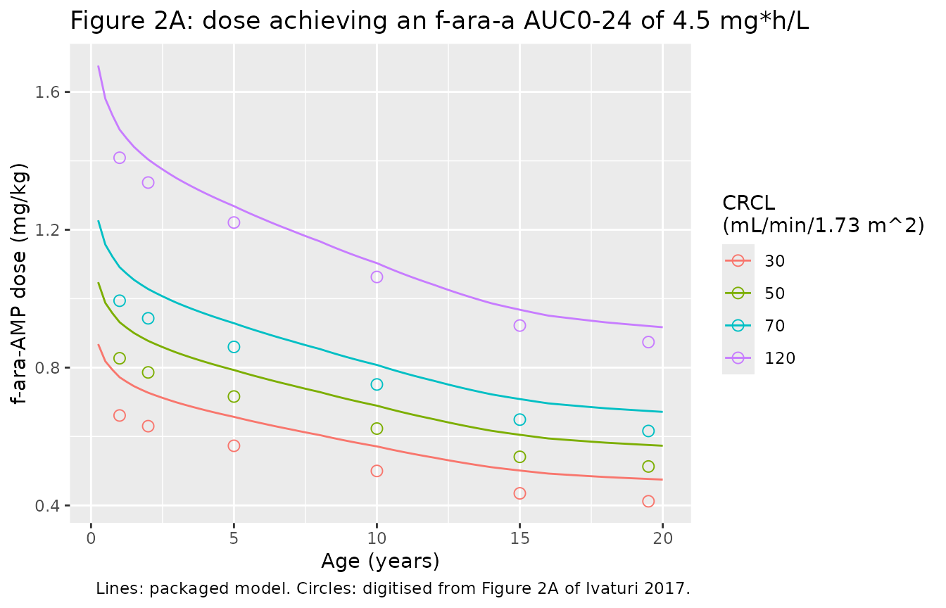
fig2_cmp <- fig2_digitised |>
  mutate(WT = wt_at(age), model_dose = 4.5 * cl_typ(WT, CRCL) * 1.28 / WT,
         pct_diff = 100 * (model_dose / fig_dose - 1))
fig2_cmp |>
  select(age, CRCL, fig_dose, model_dose, pct_diff) |>
  tidyr::pivot_wider(names_from = CRCL, values_from = c(fig_dose, model_dose, pct_diff)) |>
  dplyr::rename(
    "Age (y)" = age,
    "Fig, CRCL 120" = fig_dose_120, "Model, CRCL 120" = model_dose_120, "% diff, 120" = pct_diff_120,
    "Fig, CRCL 30" = fig_dose_30, "Model, CRCL 30" = model_dose_30, "% diff, 30" = pct_diff_30
  ) |>
  select(`Age (y)`, `Fig, CRCL 120`, `Model, CRCL 120`, `% diff, 120`, `Fig, CRCL 30`, `Model, CRCL 30`, `% diff, 30`) |>
knitr::kable(digits = 2, caption = "Figure 2A digitised vs packaged model (f-ara-AMP mg/kg).")| Age (y) | Fig, CRCL 120 | Model, CRCL 120 | % diff, 120 | Fig, CRCL 30 | Model, CRCL 30 | % diff, 30 |
|---|---|---|---|---|---|---|
| 1.0 | 1.41 | 1.49 | 5.79 | 0.66 | 0.77 | 16.78 |
| 2.0 | 1.34 | 1.40 | 5.01 | 0.63 | 0.73 | 15.40 |
| 5.0 | 1.22 | 1.27 | 3.90 | 0.57 | 0.66 | 14.65 |
| 10.0 | 1.06 | 1.10 | 3.78 | 0.50 | 0.57 | 14.26 |
| 15.0 | 0.92 | 0.97 | 4.98 | 0.44 | 0.50 | 15.23 |
| 19.5 | 0.87 | 0.92 | 5.33 | 0.41 | 0.48 | 15.71 |
# Structural gate: clearance, its weight exponent and the reference weight set
# the CRCL 120 curve; a transcription error there moves it by tens of percent.
stopifnot(all(abs(fig2_cmp$pct_diff[fig2_cmp$CRCL == 120]) < 12))
stopifnot(all(abs(fig2_cmp$pct_diff) < 20))
The CRCL 120 curve agrees within about 6% at every age, which is within what the CDC weight approximation allows. The low-CRCL curves are 10-17% higher than the figure. Their ratio to the CRCL 120 curve is the same at every age in the figure (30/120 = 0.47, 50/120 = 0.59, 70/120 = 0.71), as the model structure predicts. Solving those three ratios for CRCLEFF gives 0.0067 each time, against the printed 0.006:
ratio_fig <- fig2_digitised |>
  group_by(age) |>
  mutate(ratio = fig_dose / fig_dose[CRCL == 120]) |>
  ungroup() |>
  filter(CRCL != 120) |>
  group_by(CRCL) |>
  summarise(ratio = mean(ratio), .groups = "drop") |>
  mutate(implied_crcleff = (1 - ratio) / ((100 - CRCL) + ratio * 20))
knitr::kable(ratio_fig, digits = 4, caption = "CRCLEFF implied by the Figure 2A curve ratios.")| CRCL | ratio | implied_crcleff |
|---|---|---|
| 30 | 0.4705 | 0.0067 |
| 50 | 0.5868 | 0.0067 |
| 70 | 0.7051 | 0.0067 |
The figure was presumably drawn with the unrounded estimate, which the table’s ‘.006’ does not resolve to a second significant figure (its bootstrap 95% CI is .004-.008). The packaged model keeps the printed 0.006. At CRCL 30 this gives a clearance about 10% higher than the figure implies. Above 100 the difference is under 1%.
The ‘Schwartz’ curve of Figure 2 is not reproduced. It depends on which Schwartz constant, height reference and CRCL cap the authors used, and the paper does not state these.
Virtual cohort
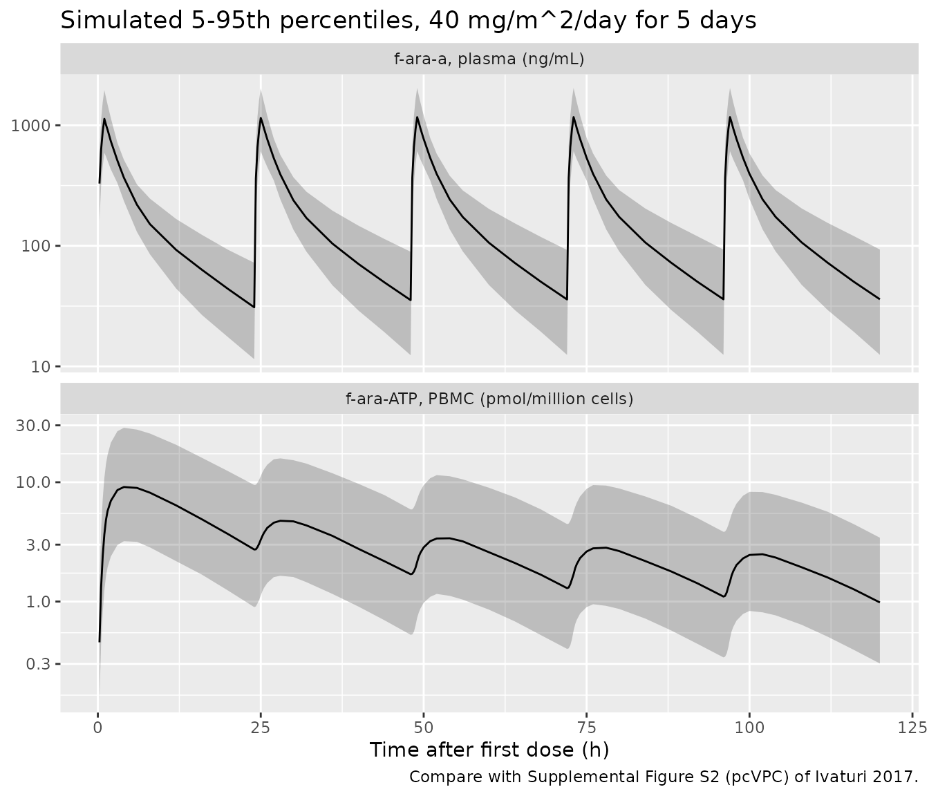
Observed data are not public. The cohort approximates Table 1, with everyone dosed at the most common regimen, 40 mg/m^2/day fludarabine phosphate. Age is drawn from a piecewise-linear quantile function anchored at the minimum (0.2 years), the median (5.0 years) and the maximum (17.9 years). The upper quartile is placed at 10 years. Weight and height are CDC medians at that age with lognormal scatter. BSA uses the Mosteller formula. CRCL is drawn lognormal around 165 mL/min/1.73 m^2 and capped at 150, so that, as in Table 1, more than half the cohort sits at the cap.
set.seed(2017)
rxode2::rxSetSeed(2017)
n_sub <- 200L

age_p <- c(0, 0.25, 0.50, 0.75, 1)
age_q <- c(0.2, 1.5, 5.0, 10.0, 17.9)

cohort <- tibble::tibble(
  id = seq_len(n_sub),
  AGE = stats::approx(age_p, age_q, xout = stats::runif(n_sub))$y
) |>
  mutate(
    WT = wt_at(AGE) * exp(stats::rnorm(n_sub, 0, 0.15)),
    HT = ht_at(AGE) * exp(stats::rnorm(n_sub, 0, 0.04)),
    BSA = sqrt(HT * WT / 3600),
    CRCL = pmin(150, 165 * exp(stats::rnorm(n_sub, 0, 0.35))),
    dose_famp = 40 * BSA,
    amt = dose_famp * 285 / 365,
    treatment = "40 mg/m^2"
  )

tibble::tibble(
  Characteristic = c("Age (years)", "Weight (kg)", "BSA (m^2)", "CRCL (mL/min/1.73 m^2)", "Fraction at CRCL cap"),
  Simulated = c(
    sprintf("%.1f (%.1f-%.1f)", median(cohort$AGE), min(cohort$AGE), max(cohort$AGE)),
    sprintf("%.1f (%.1f-%.0f)", median(cohort$WT), min(cohort$WT), max(cohort$WT)),
    sprintf("%.2f (%.2f-%.2f)", median(cohort$BSA), min(cohort$BSA), max(cohort$BSA)),
    sprintf("%.0f (%.0f-%.0f)", median(cohort$CRCL), min(cohort$CRCL), max(cohort$CRCL)),
    sprintf("%.0f%%", 100 * mean(cohort$CRCL >= 150))
  ),
  `Table 1` = c("5.0 (0.2-17.9)", "15.7 (3-111)", "0.68 (0.2-2.3)", "150 (35-150)", "median at cap")
) |>
knitr::kable(caption = "Virtual cohort vs Table 1 (median and range).")| Characteristic | Simulated | Table 1 |
|---|---|---|
| Age (years) | 4.5 (0.2-17.9) | 5.0 (0.2-17.9) |
| Weight (kg) | 17.4 (5.4-69) | 15.7 (3-111) |
| BSA (m^2) | 0.70 (0.30-1.83) | 0.68 (0.2-2.3) |
| CRCL (mL/min/1.73 m^2) | 150 (64-150) | 150 (35-150) |
| Fraction at CRCL cap | 66% | median at cap |
Five daily doses are given, each a 1-hour infusion of the f-ara-a
equivalent of the fludarabine phosphate dose. Observations are on the
plasma state (cmt = "central") with dvid = 1;
the model returns both Cc and Cpbmc_faraatp at
every observation row.
n_dose <- 5L
dur_inf <- 1
obs_day <- c(0, 0.25, 0.5, 0.75, 1, 1.25, 1.5, 2, 3, 4, 6, 8, 12, 16, 20, 24)
obs_times <- sort(unique(as.vector(outer(obs_day, 24 * (seq_len(n_dose) - 1), "+"))))

doses <- cohort |>
  select(id, amt, WT, CRCL, treatment) |>
  tidyr::crossing(dose_num = seq_len(n_dose)) |>
  mutate(time = 24 * (dose_num - 1), rate = amt / dur_inf, evid = 1L, cmt = "central", dvid = NA_integer_) |>
  select(-dose_num)

obs <- cohort |>
  select(id, WT, CRCL, treatment) |>
  tidyr::crossing(time = obs_times) |>
  mutate(amt = 0, rate = 0, evid = 0L, cmt = "central", dvid = 1L)

events <- bind_rows(doses, obs) |>
  arrange(id, time, desc(evid)) |>
  as.data.frame()
stopifnot(!anyDuplicated(events[, c("id", "time", "evid")]))
Simulation
sim <- rxode2::rxSolve(mod, events = events, keep = c("treatment", "WT", "CRCL")) |>
  as.data.frame()
#> ℹ parameter labels from comments will be replaced by 'label()'
vpc <- sim |>
  select(time, Cc, Cpbmc_faraatp) |>
  tidyr::pivot_longer(-time, names_to = "analyte", values_to = "value") |>
  filter(time > 0) |>
  group_by(analyte, time) |>
  summarise(
    Q05 = quantile(value, 0.05), Q50 = median(value), Q95 = quantile(value, 0.95),
    .groups = "drop"
  ) |>
  mutate(analyte = recode(analyte,
    Cc = "f-ara-a, plasma (ng/mL)",
    Cpbmc_faraatp = "f-ara-ATP, PBMC (pmol/million cells)"
  ))

ggplot(vpc, aes(time, Q50)) +
  geom_ribbon(aes(ymin = Q05, ymax = Q95), alpha = 0.25) +
  geom_line() +
  facet_wrap(~analyte, ncol = 1, scales = "free_y") +
  scale_y_log10() +
  labs(
    x = "Time after first dose (h)", y = NULL,
    title = "Simulated 5-95th percentiles, 40 mg/m^2/day for 5 days",
    caption = "Compare with Supplemental Figure S2 (pcVPC) of Ivaturi 2017."
  )
PKNCA: f-ara-a daily exposure (Table 4)
Table 4 reports the observed f-ara-a AUC0-24 for patients on 40 mg/m^2/dose as a median of 4.5 mgh/L (4500 ngh/mL). The Methods also use 4.5 mg*h/L as the target derived from that group. The NCA below uses the first dosing interval.
nca_conc <- sim |>
  filter(!is.na(Cc), time <= 24) |>
  select(id, time, Cc, treatment)
nca_conc <- bind_rows(
  nca_conc,
  nca_conc |> distinct(id, treatment) |> mutate(time = 0, Cc = 0)
) |>
  distinct(id, treatment, time, .keep_all = TRUE) |>
  arrange(id, treatment, time)

nca_dose <- doses |>
  filter(time == 0) |>
  select(id, time, amt, treatment)

conc_obj <- PKNCA::PKNCAconc(nca_conc, Cc ~ time | treatment + id)
dose_obj <- PKNCA::PKNCAdose(nca_dose, amt ~ time | treatment + id)
intervals <- data.frame(start = 0, end = 24, cmax = TRUE, tmax = TRUE, auclast = TRUE)
nca_res <- PKNCA::pk.nca(PKNCA::PKNCAdata(conc_obj, dose_obj, intervals = intervals))

published <- tibble::tribble(
  ~treatment, ~auclast,
  "40 mg/m^2", 4500
)
cmp <- nlmixr2lib::ncaComparisonTable(
  simulated = nca_res,
  reference = published,
  by = "treatment",
  units = c(auclast = "ng*h/mL", cmax = "ng/mL", tmax = "h"),
  tolerance_pct = 20
)
knitr::kable(cmp, caption = "Simulated vs published f-ara-a AUC0-24 at 40 mg/m^2 (Table 4). * differs by >20%.")| NCA parameter | treatment | Reference | Simulated | % diff |
|---|---|---|---|---|
| AUClast (ng*h/mL) | 40 mg/m^2 | 4500 | 4670 | +3.7% |
auc_med <- median(as.data.frame(nca_res)$PPORRES[as.data.frame(nca_res)$PPTESTCD == "auclast"])
stopifnot(abs(auc_med / 4500 - 1) < 0.2)
The simulated median is close to the observed 4.5 mg*h/L. The paper does not give the age or weight distribution of the 55 patients dosed at 40 mg/m^2. The cohort here applies that regimen to the whole Table 1 population, including the youngest children, who were mostly dosed by mg/kg.
A closed-form check confirms that the ODE solution conserves dose: the AUC from time zero to infinity after one dose equals dose / CL.
one <- data.frame(
  id = 1, time = c(0, seq(0, 400, by = 0.25)), amt = c(20, rep(0, 1601)),
  rate = c(20, rep(0, 1601)), evid = c(1L, rep(0L, 1601)), cmt = "central",
  dvid = c(NA_integer_, rep(1L, 1601)), WT = 15, CRCL = 100
)
one_typ <- rxode2::rxSolve(rxode2::zeroRe(mod), events = one) |> as.data.frame()
#> ℹ parameter labels from comments will be replaced by 'label()'
#> ℹ omega/sigma items treated as zero: 'etalcl', 'etalvc', 'etalkmet_faraatp'
auc_ode <- sum(diff(one_typ$time) * (head(one_typ$Cc, -1) + tail(one_typ$Cc, -1)) / 2) / 1000
auc_cf <- 20 / cl_typ(15, 100)
c(ode_mg_h_L = auc_ode, dose_over_cl = auc_cf)
#>   ode_mg_h_L dose_over_cl
#>     6.451613     6.451613
stopifnot(abs(auc_ode / auc_cf - 1) < 0.01)
f-ara-ATP: Table 3 and the time effect
Table 3 lists observed median f-ara-ATP at 2 h and 24 h after the start of each dose. The cells with at least 22 samples are doses 1, 3 and 4. The cohort’s simulated medians at the same times:
table3 <- tibble::tribble(
  ~dose_num, ~tad_h, ~observed, ~n_obs,
  1, 2, 7.9, 27, 2, 2, 1.5, 4, 3, 2, 3.4, 22, 4, 2, 1.7, 28, 5, 2, 0.6, 5,
  1, 24, 2.0, 33, 2, 24, 0.5, 12, 3, 24, 1.0, 25, 4, 24, 0.9, 31, 5, 24, 0.5, 6
)

# The 24 h value of dose d is the pre-dose value of dose d + 1.
sim_atp <- tidyr::crossing(dose_num = seq_len(n_dose), tad_h = c(2, 24)) |>
  mutate(time = 24 * (dose_num - 1) + tad_h) |>
  left_join(
    sim |> group_by(time) |> summarise(simulated = median(Cpbmc_faraatp), .groups = "drop"),
    by = "time"
  ) |>
  select(-time)

t3 <- table3 |>
  left_join(sim_atp, by = c("dose_num", "tad_h")) |>
  mutate(ratio = simulated / observed)
t3 |>
  dplyr::rename(
    "Dose" = dose_num, "Hours after start of infusion" = tad_h,
    "Observed median" = observed, "Samples" = n_obs,
    "Simulated median" = simulated, "Simulated / observed" = ratio
  ) |>
knitr::kable(digits = 2, caption = "f-ara-ATP (pmol/million cells): Table 3 vs simulation at 40 mg/m^2.")| Dose | Hours after start of infusion | Observed median | Samples | Simulated median | Simulated / observed |
|---|---|---|---|---|---|
| 1 | 2 | 7.9 | 27 | 6.99 | 0.88 |
| 2 | 2 | 1.5 | 4 | 4.15 | 2.77 |
| 3 | 2 | 3.4 | 22 | 2.85 | 0.84 |
| 4 | 2 | 1.7 | 28 | 2.32 | 1.36 |
| 5 | 2 | 0.6 | 5 | 2.02 | 3.37 |
| 1 | 24 | 2.0 | 33 | 2.73 | 1.37 |
| 2 | 24 | 0.5 | 12 | 1.69 | 3.39 |
| 3 | 24 | 1.0 | 25 | 1.30 | 1.30 |
| 4 | 24 | 0.9 | 31 | 1.10 | 1.22 |
| 5 | 24 | 0.5 | 6 | 0.98 | 1.97 |
well <- t3 |> filter(n_obs >= 20)
# Centre and envelope only: the Kin variability is 82% CV and the observed
# medians come from 22-33 samples on mixed regimens.
stopifnot(
  median(abs(log(well$ratio))) < log(1.5),
  all(abs(log(well$ratio)) < log(2))
)
The well-sampled cells agree within a factor of about 1.4. The dose-2 and dose-5 cells hold only 4-12 samples. They are over-predicted about threefold and are left out of the check.
The time effect’s functional form is not printed. For each candidate form, the typical subject (15.7 kg, CRCL 150 mL/min/1.73 m^2, 40 mg/m^2 over 1 h) is solved with the printed Kin = 0.005 and exponent -0.41. The solve uses a small stand-alone ODE so that the forms differ only in how Kin changes with time.
alt <- rxode2::rxode2({
  cl <- 3.1 * (WT / 15)^0.75 * (1 + (CRCL - 100) * 0.006)
  vc <- 13.4 * WT / 15
  vp <- 13.4 * WT / 15
  q <- 2.2 * (WT / 15)^0.75
  n <- floor(t / 24) + 1
  tpos <- max(t, 1e-4)
  kt <- 1
  if (form == 1) kt <- tpos^(-0.41)
  if (form == 2) kt <- exp(-0.41 * (n - 1))
  if (form == 3) kt <- n^(-0.41)
  if (form == 4) kt <- exp(-0.41 * t / 24)
  cp <- central / vc * 1000
  d/dt(central) <- -cl / vc * central - q / vc * central + q / vp * peripheral1
  d/dt(peripheral1) <- q / vc * central - q / vp * peripheral1
  d/dt(atp) <- 0.005 * kt * cp - 0.09 * atp
})

typ_wt <- 15.7
# Table 1 medians: 15.7 kg, BSA 0.68 m^2.
typ_amt <- 40 * 0.68 * 285 / 365
typ_ev <- rxode2::et(amt = typ_amt, dur = 1, cmt = "central", ii = 24, addl = 4) |>
  rxode2::et(c(2, 24, 50, 72, 74, 96))
forms <- c(
  "Kin * TAFD^-0.41 (packaged)" = 1, "Kin * exp(-0.41 (dose - 1))" = 2,
  "Kin * dose^-0.41" = 3, "Kin * exp(-0.41 TAFD/24)" = 4, "constant Kin" = 0
)
form_tab <- lapply(names(forms), function(nm) {
  s <- as.data.frame(rxode2::rxSolve(alt, typ_ev, params = c(WT = typ_wt, CRCL = 150, form = forms[[nm]])))
  tibble::tibble(form = nm, time = s$time, atp = s$atp)
}) |> bind_rows()

obs_cells <- tibble::tibble(
  time = c(2, 24, 50, 72, 74, 96),
  cell = c("dose 1, 2 h", "dose 1, 24 h", "dose 3, 2 h", "dose 3, 24 h", "dose 4, 2 h", "dose 4, 24 h"),
  observed = c(7.9, 2.0, 3.4, 1.0, 1.7, 0.9)
)
form_cmp <- form_tab |>
  inner_join(obs_cells, by = "time") |>
  group_by(form) |>
  mutate(med_abs_log = median(abs(log(atp / observed)))) |>
  ungroup()
form_cmp |>
  select(form, cell, atp) |>
  tidyr::pivot_wider(names_from = cell, values_from = atp) |>
  left_join(form_cmp |> distinct(form, med_abs_log), by = "form") |>
  mutate(`Median fold error` = exp(med_abs_log)) |>
  select(-med_abs_log) |>
  bind_rows(tibble::tibble(form = "Observed (Table 3)", !!!setNames(as.list(obs_cells$observed), obs_cells$cell))) |>
knitr::kable(digits = 2, caption = "Typical f-ara-ATP (pmol/million cells) under candidate time-effect forms vs Table 3.")| form | dose 1, 2 h | dose 1, 24 h | dose 3, 2 h | dose 3, 24 h | dose 4, 2 h | dose 4, 24 h | Median fold error |
|---|---|---|---|---|---|---|---|
| Kin * TAFD^-0.41 (packaged) | 7.74 | 2.85 | 2.99 | 1.27 | 2.42 | 1.08 | 1.23 |
| Kin * exp(-0.41 (dose - 1)) | 7.61 | 5.18 | 7.06 | 2.97 | 4.79 | 1.99 | 2.39 |
| Kin * dose^-0.41 | 7.61 | 5.18 | 9.03 | 4.14 | 7.92 | 3.67 | 3.29 |
| Kin * exp(-0.41 TAFD/24) | 7.46 | 4.47 | 6.49 | 2.56 | 4.40 | 1.71 | 2.07 |
| constant Kin | 7.61 | 5.18 | 13.04 | 6.34 | 13.18 | 6.36 | 4.93 |
| Observed (Table 3) | 7.90 | 2.00 | 3.40 | 1.00 | 1.70 | 0.90 | NA |
fold <- form_cmp |> distinct(form, med_abs_log)
stopifnot(
  fold$med_abs_log[fold$form == "Kin * TAFD^-0.41 (packaged)"] ==
    min(fold$med_abs_log)
)
Only the power-of-time form fits all three doses. The per-dose and per-day exponential forms put the dose-1 24-hour trough 2.2-2.6 times above the observed median, because they hold Kin constant through the whole first day. The same feature appears in the individual fits of Figure 1B, where f-ara-ATP falls to about 0.3 of its dose-1 peak by 24 hours.
The packaged model computes time after the first dose with
tafd(central). Its typical-value solution matches the
stand-alone power-of-time ODE:
pk_ev <- data.frame(
  id = 1, time = c(24 * 0:4, 2, 24, 50, 72, 74, 96), amt = c(rep(typ_amt, 5), rep(0, 6)),
  rate = c(rep(typ_amt, 5), rep(0, 6)), evid = c(rep(1L, 5), rep(0L, 6)), cmt = "central",
  dvid = c(rep(NA_integer_, 5), rep(1L, 6)), WT = typ_wt, CRCL = 150
) |> arrange(time, desc(evid))
pk_typ <- rxode2::rxSolve(rxode2::zeroRe(mod), events = pk_ev) |> as.data.frame()
#> ℹ parameter labels from comments will be replaced by 'label()'
#> ℹ omega/sigma items treated as zero: 'etalcl', 'etalvc', 'etalkmet_faraatp'
ref <- form_tab |> filter(form == "Kin * TAFD^-0.41 (packaged)")
cross <- tibble::tibble(time = pk_typ$time, packaged = pk_typ$Cpbmc_faraatp) |>
  inner_join(ref |> select(time, standalone = atp), by = "time")
knitr::kable(cross, digits = 4)| time | packaged | standalone |
|---|---|---|
| 2 | 7.7387 | 7.7387 |
| 24 | 2.8481 | 2.8481 |
| 50 | 2.9929 | 2.9929 |
| 72 | 1.2677 | 1.2677 |
| 74 | 2.4152 | 2.4152 |
| 96 | 1.0761 | 1.0761 |
f-ara-ATP NCA after the first dose
atp_conc <- sim |>
  filter(!is.na(Cpbmc_faraatp), time <= 24) |>
  select(id, time, Cpbmc_faraatp, treatment)
atp_obj <- PKNCA::PKNCAconc(atp_conc, Cpbmc_faraatp ~ time | treatment + id)
atp_res <- PKNCA::pk.nca(PKNCA::PKNCAdata(atp_obj, dose_obj,
  intervals = data.frame(start = 0, end = 24, cmax = TRUE, tmax = TRUE, auclast = TRUE)
))
summary(atp_res)
#>  start end treatment   N    auclast        cmax              tmax
#>      0  24 40 mg/m^2 200 145 [77.6] 9.34 [75.5] 4.00 [4.00, 6.00]
#>
#> Caption: auclast, cmax: geometric mean and geometric coefficient of variation; tmax: median and range; N: number of subjects
The paper reports no NCA for f-ara-ATP. The simulated dose-1 peak occurs a few hours after the start of infusion, consistent with the individual fits in Figure 1B.
Variability scale
Table 2 prints each IIV row as a percentage labelled %CV, with an RSE and a bootstrap 95% CI. Two readings compete:
- The percentage is omega x 100, so omega^2 = (P/100)^2.
- The percentage is a true CV, so omega^2 = log(1 + CV^2).
Each reading implies a different RSE of omega from the CI. Only the first reproduces the printed RSEs on the wide rows, where the two readings differ.
iiv <- tibble::tribble(
  ~row, ~P, ~rse_printed, ~lower, ~upper,
  "CL", 31.7, 7.8, 26.4, 36.0,
  "Vc", 38.3, 21.9, 24.4, 56.1,
  "Kin", 81.9, 10.8, 60.0, 97.6
)
implied_rse <- function(P, L, U, tr) {
  ((tr(U / 100) - tr(L / 100)) / 2) / tr(P / 100) / 1.96 * 100 / 2
}
iiv |>
  mutate(
    sd_reading = implied_rse(P, lower, upper, function(x) x^2),
    cv_reading = implied_rse(P, lower, upper, function(x) log(1 + x^2))
  ) |>
  dplyr::rename(
    "IIV row" = row, "Printed value" = P, "Printed RSE (%)" = rse_printed,
    "CI lower" = lower, "CI upper" = upper,
    "Implied RSE, omega x 100" = sd_reading, "Implied RSE, log(1 + CV^2)" = cv_reading
  ) |>
knitr::kable(digits = 1, caption = "RSE of omega implied by the Table 2 bootstrap CI under each reading.")| IIV row | Printed value | Printed RSE (%) | CI lower | CI upper | Implied RSE, omega x 100 | Implied RSE, log(1 + CV^2) |
|---|---|---|---|---|---|---|
| CL | 31.7 | 7.8 | 26.4 | 36.0 | 7.6 | 7.3 |
| Vc | 38.3 | 21.9 | 24.4 | 56.1 | 22.2 | 20.1 |
| Kin | 81.9 | 10.8 | 60.0 | 97.6 | 11.3 | 9.0 |
The packaged model uses omega^2 = (P/100)^2. The Kin variance is 0.671. The log(1 + CV^2) conversion would give 0.513.
Assumptions and deviations
-
Kin time effect. The functional form is not
printed. It is encoded as a power of time after the first dose in hours,
Kin(t) = 0.005 x TAFD^-0.41, as justified above. The value at TAFD = 1 h is the printed 0.005. TAFD is floored at 1e-4 h so the power stays finite at the moment of the first dose, where the plasma concentration, and so the uptake flux, is zero. - f-ara-ATP input. Kin multiplies the plasma f-ara-a concentration in ng/mL. This is the only reading that gives f-ara-ATP in the assay’s pmol per million cells at the observed magnitude. The uptake removes no f-ara-a from plasma; the paper models the PBMC pool as a separate per-cell quantity.
- Units in Table 2. Vc is printed as ‘L/kg’ and Q as ‘L/h/kg’, while CL is ‘L/h/15 kg’ and Vp ‘L/15’. Read literally, 13.4 L/kg would give a 15 kg child a 201 L central volume and f-ara-a peaks about 15-fold below the ~1000 ng/mL of Figure 1A. All four are taken per 15 kg.
- Allometric exponents. Only the CL exponent (0.75) is printed. Q uses 0.75 and Vc and Vp use 1, the standard allometric values.
- CRCLEFF. The printed 0.006 is kept, although Figure 2’s curve ratios imply about 0.0067 (see Figure 2 above). Doses for children with CRCL well below 100 mL/min/1.73 m^2 therefore come out up to about 17% above Figure 2.
-
CRCL cap. The estimation data were capped at 150
mL/min/1.73 m^2 (Table 1 range; stated explicitly by Brooks 2022). The
cap is documented in the model’s covariate notes and should be applied
to CRCL before simulation. It is not applied inside
model(). -
Variability scale. Table 2 labels the IIV
percentages %CV. They are taken as omega x 100, so omega^2 = (P/100)^2.
The printed RSEs decide this. For each row, the RSE of omega implied by
the bootstrap 95% CI matches the printed RSE under this reading (Kin
11.3 vs 10.8 printed, Vc 22.2 vs 21.9, CL 7.6 vs 7.8). Under omega^2 =
log(1 + CV^2) it does not (Kin 9.0, Vc 20.1, CL 7.3); see ‘Variability
scale’ above. The residual percentages are read on the same scale, as
log-scale SDs (0.248 and 0.715), and the log-scale additive error is
encoded as
lnorm(). - Infusion duration. The paper gives 30-60 minutes; the simulations use 1 hour. A 30-minute infusion raises the 2-hour f-ara-ATP value by about 20%.
- Virtual cohort. Everyone receives 40 mg/m^2/day for five days. The age quartiles other than the median and the CRCL distribution below the cap are not reported and are assumed.
- No erratum or correction notice for this article was found on PubMed or PMC as of 2026-10-17.