Salbutamol plasma and urine MBMA (Courlet 2022)

Model and source

• Citation: Courlet P, Buclin T, Biollaz J, Mazzoni I, Rabin O, Guidi M. Model-based meta-analysis of salbutamol pharmacokinetics and practical implications for doping control. CPT Pharmacometrics Syst Pharmacol. 2022;11(4):469-481. doi:10.1002/psp4.12773.
• Description: MBMA. One-compartment population PK model of salbutamol (albuterol) in plasma and urine, fitted jointly to individual and aggregate (study-mean) data from 13 published studies in healthy volunteers, trained athletes and asthmatics (Courlet 2022, WADA doping-control analysis). An inhaled dose splits into a fixed 20% lung fraction absorbed first-order from a lung depot and an 80% swallowed fraction absorbed first-order from the gut with the oral bioavailability; an oral dose enters the gut depot only. Urinary excretion of unchanged salbutamol is a first-order arm of the total clearance into a cumulative urine compartment, and the urine concentration is that amount divided by the urine volume produced at a constant rate since the last bladder voiding. Physical exercise lowers urine production by 15%; urine-production IIV differs between USG-corrected and uncorrected records; aggregate records scale every random effect by N^-0.25.
• Article: https://doi.org/10.1002/psp4.12773 (open access, with Supplementary Materials S1-S8)

Courlet et al. pooled individual and study-mean (aggregate) salbutamol plasma and urine concentrations from 13 published studies selected by the World Anti-Doping Agency (WADA), fitted a one-compartment population PK model with a urine compartment, and used it to ask how well the WADA urinary threshold (T = 1000 ng/mL) and decision limit (DL = 1200 ng/mL) separate permitted inhaled use from prohibited oral or supratherapeutic use.

mod <- readModelDb("Courlet_2022_salbutamol_mbma")
ui <- rxode2::rxode(mod)
#> ℹ parameter labels from comments will be replaced by 'label()'
#> Warning: some etas defaulted to non-mu referenced, possible parsing error: etalcl, etalurprod, etalurprod_usg
#> as a work-around try putting the mu-referenced expression on a simple line
th <- ui$theta

Population

The 13 studies (Supplementary Table S3) enrolled healthy volunteers, trained or elite athletes and asthmatics. Study-mean ages were 21-29 years and mean body weights 70-84 kg; every study was in males or did not report sex. Six studies contributed individual concentrations and the rest arithmetic-mean profiles of 8-30 subjects. The analysis used 121 plasma concentrations (43 individual, 78 mean-profile points) and 796 urine concentrations (747 individual, 49 mean-profile points). Inhaled doses were 200-1600 ug per administration (median 800 ug) and oral doses 4-12 mg (median 8 mg). Urine was measured either as free or as non-sulfated salbutamol, and as uncorrected or urine specific gravity (USG)-corrected concentrations. The total number of subjects is not stated (one study did not report its size).

str(mod()$population)
#> Warning: some etas defaulted to non-mu referenced, possible parsing error: etalcl, etalurprod, etalurprod_usg
#> as a work-around try putting the mu-referenced expression on a simple line
#> List of 10
#>  $ species       : chr "human"
#>  $ n_subjects    : int NA
#>  $ n_studies     : num 13
#>  $ age_range     : chr "Study means 21-29 years; individual data 22-45 years where reported (Table S3)"
#>  $ weight_range  : chr "Study means 70-84 kg; individual data 65-89 kg where reported (Table S3)"
#>  $ sex_female_pct: num NA
#>  $ disease_state : chr "Healthy volunteers, trained / elite athletes and asthmatics (with and without elite-athlete status); all studie"| __truncated__
#>  $ dose_range    : chr "Inhaled 200-1600 ug per administration (median 800 ug), daily 200-1600 ug; oral 4000-12000 ug per administratio"| __truncated__
#>  $ regions       : chr "Not reported (13 studies selected by WADA from the literature and WADA-funded projects)"
#>  $ notes         : chr "13 studies (Table S3): Pichon 2005 (10, aggregate), Sporer 2007 (30, aggregate), Sporer 2008 (8, aggregate), Ma"| __truncated__

Source trace

Equation / parameter	Value	Source location
lfdepot_lung (F1)	log(0.2), fixed	Table 1
logitfdepot_oral (logit F2)	-0.328, fixed	Table 1; F2 = exp(x)/(1+exp(x)) per the Table 1 legend
lka_lung (ka1)	log(31.6 1/h), fixed	Table 1
lka_oral (ka2)	log(1.47 1/h), fixed	Table 1
lvc (V3)	log(205 L)	Table 1
lkurine (k34)	log(0.0468 1/h)	Table 1
lcl (CL)	log(28 L/h)	Table 1
lurprod (UR_PROD)	log(0.0467 L/h)	Table 1
e_exercise_urprod	-0.153	Table 1, effect form (1 + physical x theta) in the legend
etalcl	0.1416 (39% CV)	Table 1
etalurprod (uncorrected)	0.4367 (74% CV)	Table 1
etalurprod_usg (USG-corrected)	0.1349 (38% CV)	Table 1
propSd	0.40	Table 1, proportional error plasma, individual
propSd_aggregate	0.77	Table 1, proportional error plasma, aggregate
propSd_urineSal	0.46	Table 1, proportional error urine, individual
addSd_urineSal	18 ng/mL	Table 1, additive error urine, individual
propSd_urineSal_aggregate	1.31	Table 1, proportional error urine, aggregate
Lung and gut depots, F1 split	n/a	Figure 1; Methods, Base structural model; S1 Equation 6
k30 = CL/V3 - k34	n/a	S1 Equation 2, CL = (k30 + k34) x V3
urineSal = urine / urine_vol, d/dt(urine_vol) = urprod	n/a	Methods, Base structural model (constant urine production, bladder voided before each dose)
Exercise on UR_PROD	n/a	Results, Covariate analysis; S1 Equation 4
Aggregate weight N_ARM^-0.25 on etas and residual SDs	n/a	Table 1 and Table S6 footnotes; Results, Model evaluation (see Errata)

Deterministic checks of the derived quantities

The paper reports several secondary quantities that follow directly from the Table 1 estimates. Each is recomputed below from the packaged model’s own ini() values.

ke <- exp(th[["lcl"]]) / exp(th[["lvc"]])
tmax_eq5 <- function(ka) (log(ka) - log(ke)) / (ka - ke) # S1 Equation 5
derived <- tibble::tibble(
  quantity = c(
    "Oral bioavailability F2",
    "Half-life (h), S1 Eq 7",
    "Tmax after inhalation, lung fraction only (h)",
    "Tmax after oral dosing (h)",
    "Urine production during exercise (L/h)",
    "Non-urinary elimination k30 (1/h)"
  ),
  model = c(
    1 / (1 + exp(-th[["logitfdepot_oral"]])),
    log(2) / ke,
    tmax_eq5(exp(th[["lka_lung"]])),
    tmax_eq5(exp(th[["lka_oral"]])),
    exp(th[["lurprod"]]) * (1 + th[["e_exercise_urprod"]]),
    ke - exp(th[["lkurine"]])
  ),
  paper = c(NA, 5, 0.17, 1.8, 0.0396, NA)
)
knitr::kable(derived, digits = 4)

quantity	model	paper
Oral bioavailability F2	0.4187	NA
Half-life (h), S1 Eq 7	5.0748	5.0000
Tmax after inhalation, lung fraction only (h)	0.1730	0.1700
Tmax after oral dosing (h)	1.7819	1.8000
Urine production during exercise (L/h)	0.0396	0.0396
Non-urinary elimination k30 (1/h)	0.0898	NA

stopifnot(
  abs(derived$model[2] - 5) < 0.1, # "a t1/2 of 5 h"
  round(derived$model[3], 2) == 0.17,
  round(derived$model[4], 1) == 1.8,
  round(derived$model[5], 4) == 0.0396,
  derived$model[6] > 0 # urinary arm is a fraction of the total clearance
)

The Results section also quotes the aggregate-data residual errors after the sample-size weighting: 46% and 40% for plasma profiles of 8 and 13 subjects, and 78% and 56% for urine profiles of 8 and 30 subjects. The model weights the unweighted Table 1 SDs by N_ARM^-0.25; the 1 / sqrt(N_ARM) weight printed in the Methods equation is shown for comparison.

agg <- tibble::tibble(
  matrix = c("plasma", "plasma", "urine", "urine"),
  N_ARM = c(8, 13, 8, 30),
  raw = 100 * c(th[["propSd_aggregate"]], th[["propSd_aggregate"]],
                th[["propSd_urineSal_aggregate"]], th[["propSd_urineSal_aggregate"]]),
  paper = c(46, 40, 78, 56)
) |>
  dplyr::mutate(
    model_N_quarter = raw / N_ARM^0.25,
    printed_eq_sqrt = raw / sqrt(N_ARM)
  )
knitr::kable(agg, digits = 1)

matrix	N_ARM	raw	paper	model_N_quarter	printed_eq_sqrt
plasma	8	77	46	45.8	27.2
plasma	13	77	40	40.6	21.4
urine	8	131	78	77.9	46.3
urine	30	131	56	56.0	23.9

# The raw SDs are themselves rounded to whole percent in Table 1, so allow 1.
stopifnot(all(abs(agg$model_N_quarter - agg$paper) <= 1))

Event-table conventions

• Inhaled dose: two dose records with the same amt at the same time, one into depot_lung and one into depot_oral, with ROUTE_ORAL = 0. The model makes 20% of the first and 80% x F2 of the second bioavailable.
• Oral dose: one record into depot_oral with ROUTE_ORAL = 1.
• Bladder voiding: an evid = 5 replacement record setting urine and urine_vol to 0. Urine concentrations are only defined after a voiding, so observations are taken strictly after it.
• Observations: two endpoints (Cc, urineSal). Observation rows carry dvid (1 = plasma, 2 = urine) with cmt left missing, so that the residual draw for that endpoint is returned in the sim column. Every observable is still returned as a column on every observation row.
• Individual-level simulation: DTYPE_AGGREGATED = 0, N_ARM = 1. The paper’s simulations are in individuals at rest with USG-corrected urine (EXERCISE = 0, USG_CORRECTED = 1).

endpoints <- ui$predDf[, c("var", "cmt")]
endpoints$dvid <- seq_len(nrow(endpoints))
stopifnot(identical(endpoints$var, c("Cc", "urineSal")))

# One subject's events for a regimen given as a data frame of dose times,
# amounts (ug) and routes. Doses repeat every 24 h for `days` days; the bladder
# is voided at every dose and at `extra_voids`; observations are at
# `obs_offsets` after the last dose on the endpoints listed in `obs_dvid`.
make_subject <- function(regimen, days, obs_offsets, obs_dvid, extra_voids = numeric(0)) {
  daily <- tidyr::expand_grid(day = seq_len(days) - 1, regimen) |>
    dplyr::mutate(time = time + 24 * day)
  last_dose <- max(daily$time)
  doses <- dplyr::bind_rows(
    daily |> dplyr::mutate(cmt = "depot_oral"),
    daily |> dplyr::filter(route == "inhaled") |> dplyr::mutate(cmt = "depot_lung")
  ) |>
    dplyr::transmute(time, amt, cmt, evid = 1L, dvid = NA_integer_,
                     ROUTE_ORAL = as.integer(route == "oral"))
  voids <- tidyr::expand_grid(time = sort(unique(c(daily$time, extra_voids))),
                              cmt = c("urine", "urine_vol")) |>
    dplyr::mutate(amt = 0, evid = 5L, dvid = NA_integer_)
  obs <- tidyr::expand_grid(time = last_dose + obs_offsets, dvid = obs_dvid) |>
    dplyr::mutate(amt = NA_real_, evid = 0L, cmt = NA_character_)
  dplyr::bind_rows(voids, doses, obs) |>
    # voiding precedes dosing precedes observation at a tied time
    dplyr::arrange(time, match(evid, c(5L, 1L, 0L)), dvid) |>
    tidyr::fill(ROUTE_ORAL, .direction = "downup") |>
    dplyr::mutate(last_dose = last_dose)
}

make_arm <- function(n, id_offset, ...) {
  one <- make_subject(...)
  tidyr::expand_grid(id = id_offset + seq_len(n), one) |>
    dplyr::mutate(EXERCISE = 0, USG_CORRECTED = 1, DTYPE_AGGREGATED = 0, N_ARM = 1)
}

inh <- function(times, amt) tibble::tibble(time = times, amt = amt, route = "inhaled")
oral <- function(times, amt) tibble::tibble(time = times, amt = amt, route = "oral")

Typical-value plasma profiles and Tmax after inhalation

After inhalation, plasma salbutamol is the sum of a fast lung-absorbed part and a slower swallowed part. The paper reports an intermediate Tmax of 1.45 h for the sum (S1 Equation 6, solved numerically).

grid <- seq(0.01, 12, by = 0.01)
typ_events <- dplyr::bind_rows(
  make_arm(1, 0L, regimen = inh(0, 800), days = 1, obs_offsets = grid, obs_dvid = 1L) |>
    dplyr::mutate(scenario = "800 ug inhaled"),
  make_arm(1, 1L, regimen = oral(0, 8000), days = 1, obs_offsets = grid, obs_dvid = 1L) |>
    dplyr::mutate(scenario = "8 mg oral")
)
typ <- rxode2::rxSolve(rxode2::zeroRe(mod), events = typ_events, keep = "scenario",
                       useLinCmt = FALSE, addDosing = FALSE) |>
  as.data.frame()
#> ℹ parameter labels from comments will be replaced by 'label()'
#> Warning: some etas defaulted to non-mu referenced, possible parsing error: etalcl, etalurprod, etalurprod_usg
#> as a work-around try putting the mu-referenced expression on a simple line
#> Warning: No sigma parameters in the model
#> Warning: some etas defaulted to non-mu referenced, possible parsing error: etalcl, etalurprod, etalurprod_usg
#> as a work-around try putting the mu-referenced expression on a simple line
#> ℹ omega/sigma items treated as zero: 'etalcl', 'etalurprod', 'etalurprod_usg'
#> Warning: multi-subject simulation without without 'omega'

tmax_typ <- typ |>
  dplyr::group_by(scenario) |>
  dplyr::summarise(Tmax = time[which.max(Cc)], Cmax = max(Cc), .groups = "drop")
knitr::kable(tmax_typ, digits = 3,
             caption = "Typical-value Tmax (h) and Cmax (ng/mL) after a single dose.")

Typical-value Tmax (h) and Cmax (ng/mL) after a single dose.

scenario	Tmax	Cmax
8 mg oral	1.78	12.810
800 ug inhaled	1.46	1.654

stopifnot(
  abs(tmax_typ$Tmax[tmax_typ$scenario == "800 ug inhaled"] - 1.45) < 0.05,
  abs(tmax_typ$Tmax[tmax_typ$scenario == "8 mg oral"] - 1.8) < 0.05
)

ggplot(typ, aes(time, Cc, colour = scenario)) +
  geom_line() +
  labs(x = "Time after dose (h)", y = "Plasma salbutamol (ng/mL)", colour = NULL,
       title = "Typical-value plasma profiles after a single dose")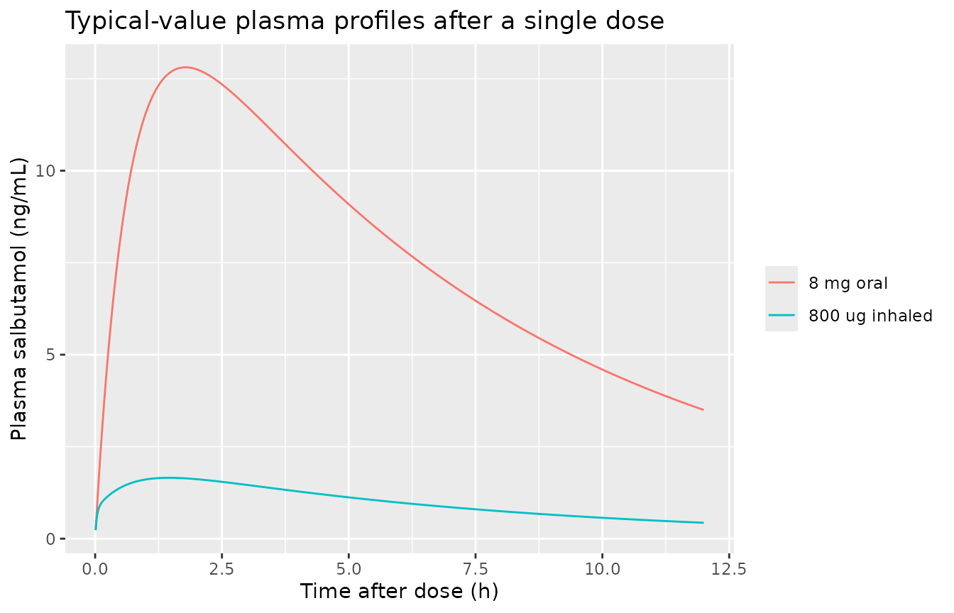

PKNCA validation of the plasma profile

A 200-subject cohort per arm receives a single 800 ug inhalation or a single 8 mg oral dose. Inter-individual variability is on clearance only, so the NCA Tmax and half-life medians should match the paper’s 1.45 h / 1.8 h and 5 h.

rxode2::rxSetSeed(20221104)
set.seed(20221104)
N_PER_ARM <- 200L
nca_grid <- c(0.05, 0.1, 0.17, 0.25, 0.5, 0.75, 1, 1.25, 1.5, 1.75, 2, 2.5, 3, 4, 6, 8, 12, 16, 24)
nca_events <- dplyr::bind_rows(
  make_arm(N_PER_ARM, 0L, regimen = inh(0, 800), days = 1, obs_offsets = nca_grid, obs_dvid = 1L) |>
    dplyr::mutate(treatment = "800 ug inhaled"),
  make_arm(N_PER_ARM, N_PER_ARM, regimen = oral(0, 8000), days = 1, obs_offsets = nca_grid, obs_dvid = 1L) |>
    dplyr::mutate(treatment = "8 mg oral")
)
stopifnot(!anyDuplicated(unique(nca_events[, c("id", "time", "evid", "cmt", "dvid")])))

nca_sim <- rxode2::rxSolve(mod, events = nca_events, keep = "treatment",
                           useLinCmt = FALSE, addDosing = FALSE) |>
  as.data.frame()
#> ℹ parameter labels from comments will be replaced by 'label()'
#> Warning: some etas defaulted to non-mu referenced, possible parsing error: etalcl, etalurprod, etalurprod_usg
#> as a work-around try putting the mu-referenced expression on a simple line

conc_df <- nca_sim |>
  dplyr::filter(!is.na(Cc)) |>
  dplyr::select(id, time, Cc, treatment)
# Pre-dose row: extravascular, so Cc = 0 at time 0.
conc_df <- dplyr::bind_rows(
  conc_df,
  conc_df |> dplyr::distinct(id, treatment) |> dplyr::mutate(time = 0, Cc = 0)
) |>
  dplyr::distinct(id, treatment, time, .keep_all = TRUE) |>
  dplyr::arrange(id, time)

dose_df <- nca_events |>
  dplyr::filter(evid == 1L) |>
  dplyr::group_by(id, treatment, time) |>
  dplyr::summarise(amt = dplyr::first(amt), .groups = "drop")

nca_res <- PKNCA::pk.nca(PKNCA::PKNCAdata(
  PKNCA::PKNCAconc(conc_df, Cc ~ time | treatment + id),
  PKNCA::PKNCAdose(dose_df, amt ~ time | treatment + id),
  intervals = data.frame(start = 0, end = 24, cmax = TRUE, tmax = TRUE,
                         auclast = TRUE, half.life = TRUE)
))

published_nca <- tibble::tibble(
  treatment = c("800 ug inhaled", "8 mg oral"),
  tmax = c(1.45, 1.8),
  half.life = c(5, 5)
)
cmp_nca <- nlmixr2lib::ncaComparisonTable(
  simulated = nca_res,
  reference = published_nca,
  by = "treatment",
  params = c("tmax", "half.life"),
  units = c(tmax = "h", half.life = "h"),
  tolerance_pct = 20
)
knitr::kable(cmp_nca, caption = paste(
  "Median NCA Tmax and half-life vs the values quoted in the Results",
  "(Tmax 1.45 h after inhalation, 1.8 h oral; t1/2 5 h).", attr(cmp_nca, "footnote")
))

Median NCA Tmax and half-life vs the values quoted in the Results (Tmax 1.45 h after inhalation, 1.8 h oral; t1/2 5 h).

NCA parameter	treatment	Reference	Simulated	% diff
Tmax (h)	800 ug inhaled	1.45	1.5	+3.4%
Tmax (h)	8 mg oral	1.8	1.75	-2.8%
t½ (h)	800 ug inhaled	5	4.91	-1.8%
t½ (h)	8 mg oral	5	4.99	-0.2%

nca_med <- as.data.frame(nca_res$result) |>
  dplyr::filter(PPTESTCD %in% c("tmax", "half.life")) |>
  dplyr::group_by(treatment, PPTESTCD) |>
  dplyr::summarise(med = median(PPORRES, na.rm = TRUE), .groups = "drop")
hl <- nca_med$med[nca_med$PPTESTCD == "half.life"]
stopifnot(
  length(hl) == 2L,
  all(abs(hl - 5) / 5 < 0.15),
  abs(nca_med$med[nca_med$PPTESTCD == "tmax" & nca_med$treatment == "8 mg oral"] - 1.8) <= 0.25,
  abs(nca_med$med[nca_med$PPTESTCD == "tmax" & nca_med$treatment == "800 ug inhaled"] - 1.45) <= 0.25
)

Steady-state urine concentrations (Figure 4)

Figure 4 and the Results compare the urine concentrations measured during the last dosing interval at steady state with the WADA T and DL. The bladder is voided at the last dose and not again; concentrations are USG-corrected, in individuals at rest, and include inter-individual and residual variability. The paper does not state its sampling grid, so the vignette samples every 0.25 h through the last dosing interval and reports the percentage of samples above each limit. Dosing runs for 4 days, well past five half-lives.

regimens <- list(
  "200 ug inhaled q.i.d." = list(reg = inh(c(0, 6, 12, 18), 200), tau = 6),
  "400 ug inhaled b.i.d." = list(reg = inh(c(0, 12), 400), tau = 12),
  "400 ug inhaled t.i.d." = list(reg = inh(c(0, 8, 16), 400), tau = 8),
  "400 ug inhaled q.i.d." = list(reg = inh(c(0, 6, 12, 18), 400), tau = 6),
  "600 ug inhaled b.i.d." = list(reg = inh(c(0, 12), 600), tau = 12),
  "800 ug inhaled b.i.d." = list(reg = inh(c(0, 12), 800), tau = 12),
  "400/600/600 ug inhaled at 0/8/16 h" = list(reg = inh(c(0, 8, 16), c(400, 600, 600)), tau = 8),
  "8 mg oral q.d." = list(reg = oral(0, 8000), tau = 24)
)
ss_events <- dplyr::bind_rows(lapply(seq_along(regimens), function(i) {
  r <- regimens[[i]]
  offsets <- sort(unique(c(seq(0.25, r$tau, by = 0.25), 1.5)))
  make_arm(N_PER_ARM, (i - 1L) * N_PER_ARM, regimen = r$reg, days = 4,
           obs_offsets = offsets, obs_dvid = 2L) |>
    dplyr::mutate(regimen = names(regimens)[i])
}))
stopifnot(!anyDuplicated(unique(ss_events[, c("id", "time", "evid", "cmt", "dvid")])))

ss <- rxode2::rxSolve(mod, events = ss_events, keep = c("regimen", "last_dose"),
                      useLinCmt = FALSE, addDosing = FALSE) |>
  as.data.frame() |>
  dplyr::filter(!is.na(sim)) |>
  dplyr::mutate(offset = round(time - last_dose, 3))
stopifnot(all(is.finite(ss$sim)), all(is.finite(ss$urineSal)))

exceed <- ss |>
  dplyr::group_by(regimen) |>
  dplyr::summarise(
    pct_T = 100 * mean(sim > 1000),
    pct_DL = 100 * mean(sim > 1200),
    .groups = "drop"
  )
paper_fig4 <- tibble::tribble(
  ~regimen, ~paper_T, ~paper_DL,
  "200 ug inhaled q.i.d.", 0, 0,
  "400 ug inhaled b.i.d.", 0, 0,
  "400 ug inhaled t.i.d.", NA, 0.2,
  "400 ug inhaled q.i.d.", NA, 0.6,
  "600 ug inhaled b.i.d.", 0.7, 0.3,
  "800 ug inhaled b.i.d.", 2.4, 1.2,
  "400/600/600 ug inhaled at 0/8/16 h", 1.9, 0.9,
  "8 mg oral q.d.", 66, 58
)
exceed_tab <- dplyr::left_join(paper_fig4, exceed, by = "regimen")
stopifnot(nrow(exceed_tab) == length(regimens), !anyNA(exceed_tab$pct_T))
exceed_tab |>
  dplyr::rename(
    "Regimen" = regimen,
    "Paper % > T" = paper_T, "Paper % > DL" = paper_DL,
    "Simulated % > T" = pct_T, "Simulated % > DL" = pct_DL
  ) |>
  knitr::kable(digits = 1, caption = paste(
    "Percentage of steady-state urine concentrations over the last dosing",
    "interval above the WADA threshold (1000 ng/mL) and decision limit",
    "(1200 ng/mL). Paper values from the Results text."
  ))

Percentage of steady-state urine concentrations over the last dosing interval above the WADA threshold (1000 ng/mL) and decision limit (1200 ng/mL). Paper values from the Results text.

Regimen	Paper % > T	Paper % > DL	Simulated % > T	Simulated % > DL
200 ug inhaled q.i.d.	0.0	0.0	0.2	0.0
400 ug inhaled b.i.d.	0.0	0.0	0.0	0.0
400 ug inhaled t.i.d.	NA	0.2	0.6	0.2
400 ug inhaled q.i.d.	NA	0.6	2.5	1.1
600 ug inhaled b.i.d.	0.7	0.3	0.6	0.2
800 ug inhaled b.i.d.	2.4	1.2	3.2	1.6
400/600/600 ug inhaled at 0/8/16 h	1.9	0.9	2.8	1.0
8 mg oral q.d.	66.0	58.0	72.4	64.7

# Replicates Figure 4 of Courlet 2022: median and prediction intervals of
# steady-state urine concentrations after the last dose.
fig4 <- ss |>
  dplyr::group_by(regimen, offset) |>
  dplyr::summarise(
    q005 = quantile(sim, 0.005), q025 = quantile(sim, 0.025), q10 = quantile(sim, 0.10),
    q50 = median(sim), q90 = quantile(sim, 0.90), q975 = quantile(sim, 0.975),
    q995 = quantile(sim, 0.995), .groups = "drop"
  ) |>
  dplyr::mutate(regimen = factor(regimen, levels = names(regimens)))
ggplot(fig4, aes(offset, q50)) +
  geom_ribbon(aes(ymin = q005, ymax = q995), fill = "steelblue", alpha = 0.15) +
  geom_ribbon(aes(ymin = q025, ymax = q975), fill = "steelblue", alpha = 0.25) +
  geom_ribbon(aes(ymin = q10, ymax = q90), fill = "steelblue", alpha = 0.35) +
  geom_line() +
  geom_hline(yintercept = 1000, colour = "firebrick", linetype = "dashed") +
  geom_hline(yintercept = 1200, colour = "orange", linetype = "dashed") +
  facet_wrap(~regimen, ncol = 4) +
  labs(x = "Time after last dose (h)", y = "Urine salbutamol (ng/mL, USG-corrected)",
       caption = "Median with 80%, 95% and 99% prediction intervals; 200 subjects per regimen.")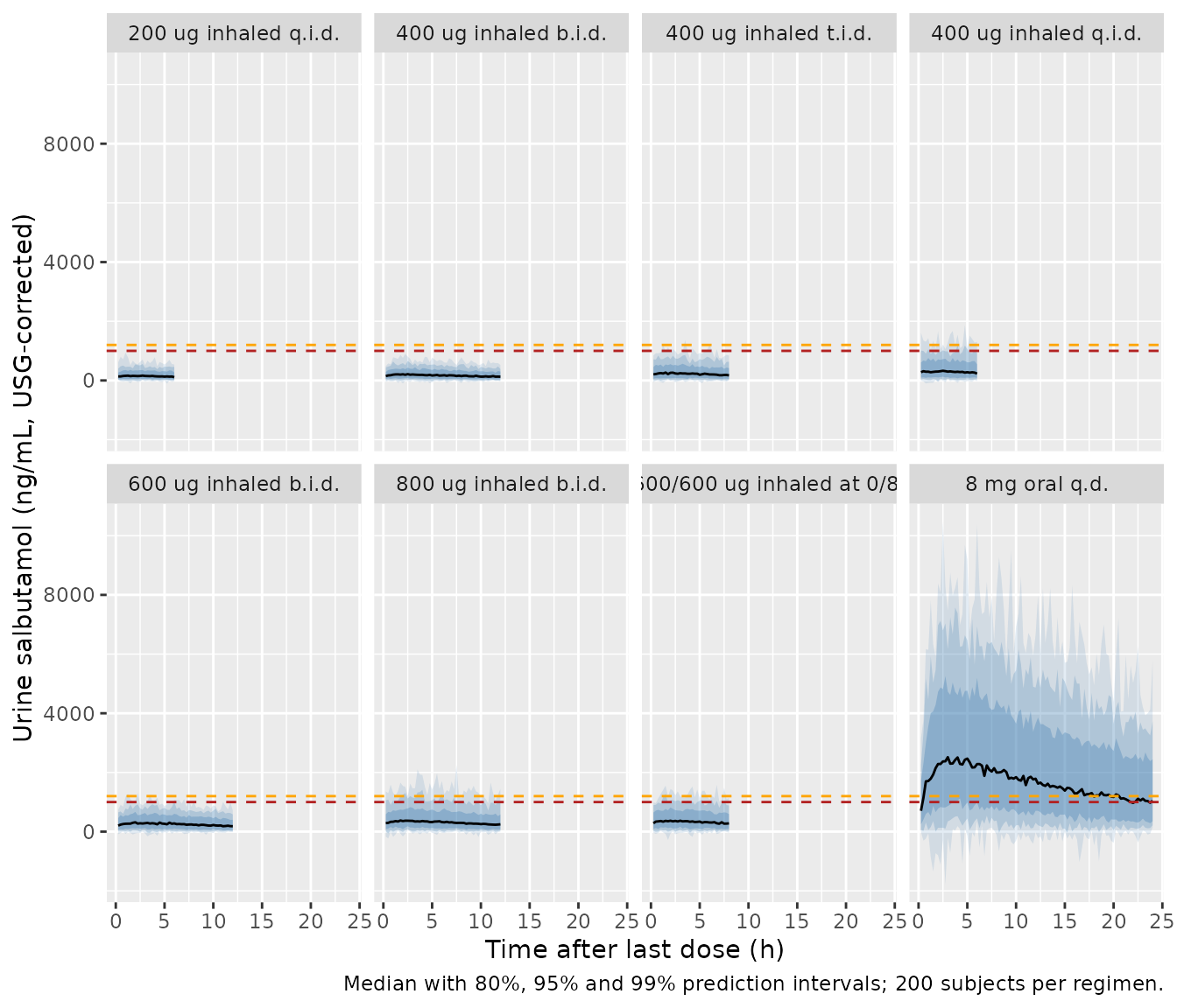

The worst-case comparison of the Results samples at the plasma Tmax (1.5 h after the last dose): the mean simulated concentration after 200 ug q.i.d. is 174 ng/mL, 4.9% (T) and 2.4% (DL) of values exceed the limits after 800 ug b.i.d., and 83% and 76% after 8 mg oral q.d. (Figure S8 part 2).

at_tmax <- ss |>
  dplyr::filter(offset == 1.5) |>
  dplyr::group_by(regimen) |>
  dplyr::summarise(mean_conc = mean(sim), pct_T = 100 * mean(sim > 1000),
                   pct_DL = 100 * mean(sim > 1200), n = dplyr::n(), .groups = "drop") |>
  dplyr::filter(regimen %in% c("200 ug inhaled q.i.d.", "800 ug inhaled b.i.d.", "8 mg oral q.d."))
paper_tmax <- tibble::tibble(
  regimen = c("200 ug inhaled q.i.d.", "800 ug inhaled b.i.d.", "8 mg oral q.d."),
  paper_mean = c(174, NA, NA), paper_T = c(0, 4.9, 83), paper_DL = c(0, 2.4, 76)
)
tmax_tab <- dplyr::left_join(paper_tmax, at_tmax, by = "regimen")
stopifnot(nrow(tmax_tab) == 3L, all(tmax_tab$n == N_PER_ARM))
knitr::kable(tmax_tab, digits = 1,
             caption = "Urine concentrations 1.5 h after the last dose at steady state.")

Urine concentrations 1.5 h after the last dose at steady state.

regimen	paper_mean	paper_T	paper_DL	mean_conc	pct_T	pct_DL	n
200 ug inhaled q.i.d.	174	0.0	0.0	175.4	0	0.0	200
800 ug inhaled b.i.d.	NA	4.9	2.4	408.7	3	1.5	200
8 mg oral q.d.	NA	83.0	76.0	2205.6	86	78.5	200

Figure 6: an arbitrary WADA-2017-compliant regimen

400 ug q.i.d. from 0 to 36 h, then 800 ug b.i.d. from 48 to 96 h, with the bladder voided every 6 h and urine sampled 2 h after the last dose. The paper reports 5.2% of concentrations above 1000 ng/mL and 2.5% above 1200 ng/mL.

fig6_reg <- inh(c(0, 6, 12, 18, 24, 30, 36, 48, 60, 72, 84, 96),
                c(rep(400, 7), rep(800, 5)))
fig6_events <- make_arm(N_PER_ARM, 0L, regimen = fig6_reg, days = 1,
                        obs_offsets = 2, obs_dvid = 2L,
                        extra_voids = seq(0, 96, by = 6))
fig6 <- rxode2::rxSolve(mod, events = fig6_events, useLinCmt = FALSE, addDosing = FALSE) |>
  as.data.frame() |>
  dplyr::filter(!is.na(sim))
stopifnot(nrow(fig6) == N_PER_ARM)
fig6_pct <- c(T = 100 * mean(fig6$sim > 1000), DL = 100 * mean(fig6$sim > 1200))
fig6_pct
#>   T  DL 
#> 2.5 2.0

ggplot(fig6, aes(sim)) +
  geom_density(fill = "grey80") +
  geom_vline(xintercept = mean(fig6$sim), colour = "blue", linetype = "dashed") +
  geom_vline(xintercept = 1000, colour = "firebrick", linetype = "dashed") +
  geom_vline(xintercept = 1200, colour = "orange", linetype = "dashed") +
  labs(x = "Urine salbutamol 2 h after the last dose (ng/mL)", y = "Density",
       title = "Replicates Figure 6 of Courlet 2022")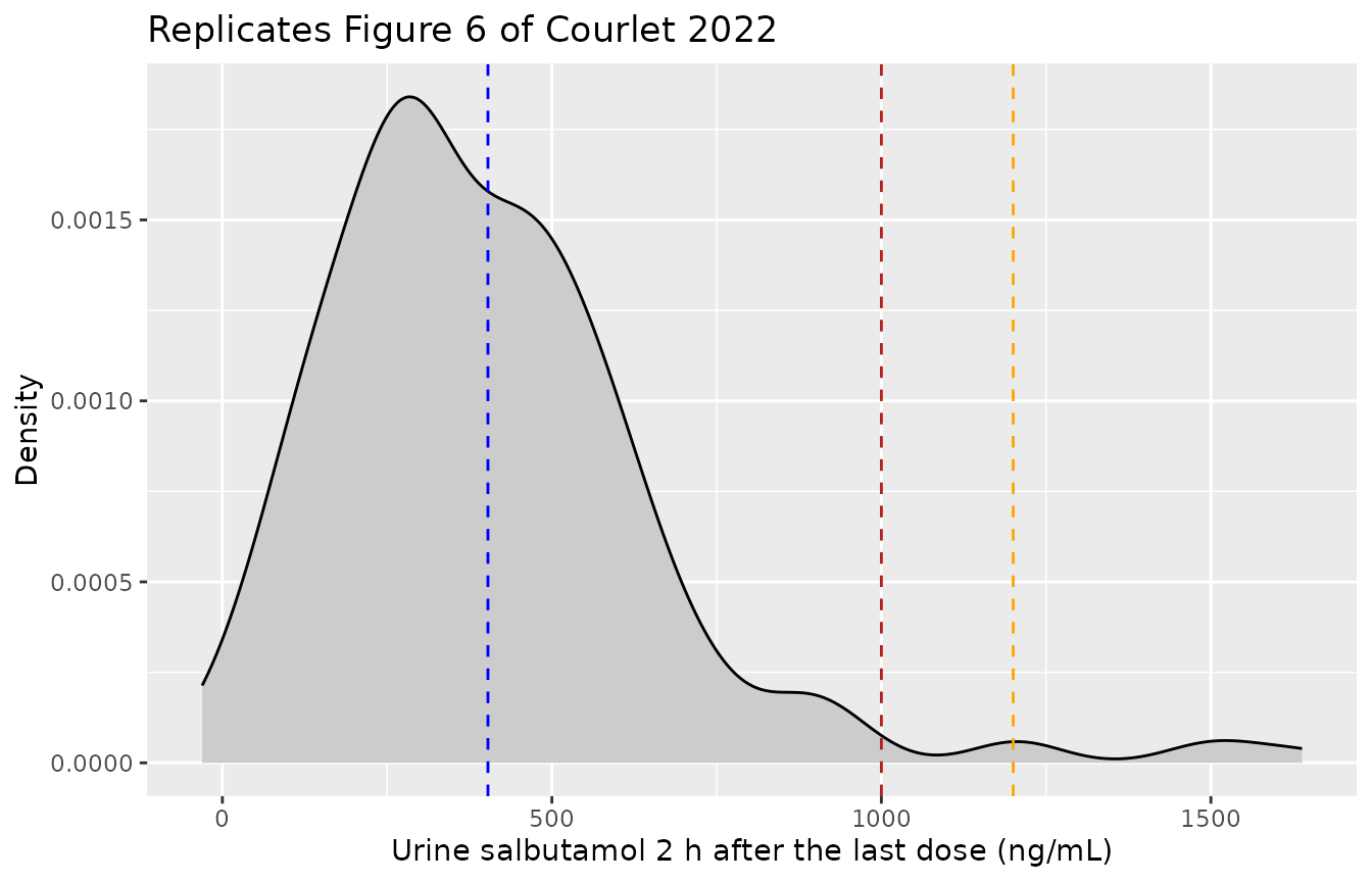

Figure 5: exercise and USG correction

Physical exercise reduces urine production by 15% and so raises the urine concentration for the same excreted amount; uncorrected urine carries the larger 74% CV on urine production instead of 38%.

conds <- tibble::tribble(
  ~condition, ~EXERCISE, ~USG_CORRECTED,
  "Reference (rest, USG-corrected)", 0, 1,
  "Physical exercise", 1, 1,
  "Without USG correction", 0, 0
)
f5_events <- dplyr::bind_rows(lapply(seq_len(nrow(conds)), function(i) {
  make_arm(N_PER_ARM, (i - 1L) * N_PER_ARM, regimen = inh(c(0, 12), 800), days = 4,
           obs_offsets = seq(0.25, 12, by = 0.25), obs_dvid = 2L) |>
    dplyr::mutate(condition = conds$condition[i], EXERCISE = conds$EXERCISE[i],
                  USG_CORRECTED = conds$USG_CORRECTED[i])
}))
f5 <- rxode2::rxSolve(mod, events = f5_events, keep = c("condition", "last_dose"),
                      useLinCmt = FALSE, addDosing = FALSE) |>
  as.data.frame() |>
  dplyr::filter(!is.na(sim)) |>
  dplyr::mutate(offset = round(time - last_dose, 3))
f5_sum <- f5 |>
  dplyr::group_by(condition, offset) |>
  dplyr::summarise(q025 = quantile(sim, 0.025), q50 = median(sim),
                   q975 = quantile(sim, 0.975), .groups = "drop")
ggplot(f5_sum, aes(offset, q50)) +
  geom_ribbon(aes(ymin = q025, ymax = q975), fill = "steelblue", alpha = 0.3) +
  geom_line() +
  geom_hline(yintercept = 1000, colour = "firebrick", linetype = "dashed") +
  geom_hline(yintercept = 1200, colour = "orange", linetype = "dashed") +
  facet_wrap(~condition) +
  labs(x = "Time after last dose (h)", y = "Urine salbutamol (ng/mL)",
       title = "800 ug inhaled b.i.d. at steady state (cf. Figure 5)")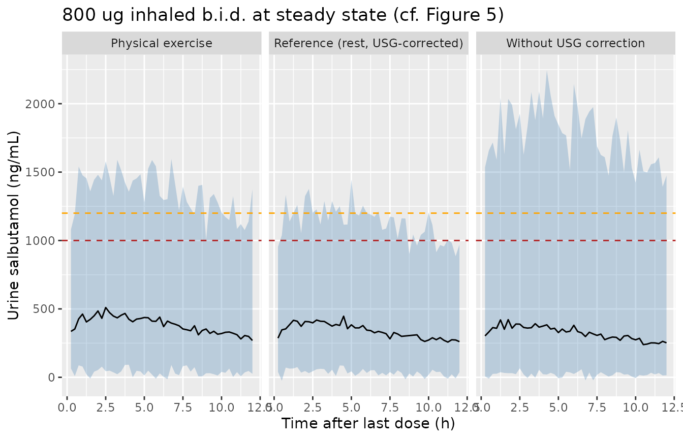

# Typical-value check: exercise scales the urine concentration by exactly
# 1 / (1 + e_exercise_urprod) = 1.18 at every time, because it acts only on
# the volume denominator.
typ5 <- rxode2::rxSolve(rxode2::zeroRe(mod),
                        events = f5_events |> dplyr::filter(id %in% c(1L, N_PER_ARM + 1L)),
                        keep = "condition", useLinCmt = FALSE, addDosing = FALSE) |>
  as.data.frame() |>
  dplyr::select(condition, time, urineSal) |>
  tidyr::pivot_wider(names_from = condition, values_from = urineSal)
#> ℹ parameter labels from comments will be replaced by 'label()'
#> Warning: some etas defaulted to non-mu referenced, possible parsing error: etalcl, etalurprod, etalurprod_usg
#> as a work-around try putting the mu-referenced expression on a simple line
#> Warning: No sigma parameters in the model
#> Warning: some etas defaulted to non-mu referenced, possible parsing error: etalcl, etalurprod, etalurprod_usg
#> as a work-around try putting the mu-referenced expression on a simple line
#> ℹ omega/sigma items treated as zero: 'etalcl', 'etalurprod', 'etalurprod_usg'
#> Warning: multi-subject simulation without without 'omega'
ratio <- typ5[["Physical exercise"]] / typ5[["Reference (rest, USG-corrected)"]]
stopifnot(all(abs(ratio - 1 / (1 + th[["e_exercise_urprod"]])) < 1e-6))

Comparison with the published simulations

The model reproduces the deterministic quantities of the paper exactly (half-life, the three Tmax values, urine production during exercise and the four weighted aggregate residual errors) and the simulated ones closely: the mean urine concentration at Tmax after 200 ug q.i.d. matches the published 174 ng/mL, the inhaled regimens give the same low single-digit exceedance percentages, and the oral 8 mg q.d. regimen sits a few points above the published 66% / 58%, a difference within what the unstated sampling grid and a 200-subject cohort allow.

pct <- function(r, col) exceed_tab[[col]][exceed_tab$regimen == r]
stopifnot(
  # Oral 8 mg q.d.: the bulk of concentrations lie above both limits. The
  # simulated values sit about 6 points above the paper's (72 / 65 at 16
  # threads), which depends on the unstated sampling grid; 15 admits that
  # offset plus cohort noise. A mis-transcribed CL, k34, UR_PROD or F2 moves
  # these by tens of points.
  abs(pct("8 mg oral q.d.", "pct_T") - 66) < 15,
  abs(pct("8 mg oral q.d.", "pct_DL") - 58) < 15,
  # Therapeutic inhaled dosing stays essentially below the limits.
  pct("200 ug inhaled q.i.d.", "pct_DL") < 1,
  pct("400 ug inhaled b.i.d.", "pct_DL") < 1,
  # 800 ug b.i.d. (WADA 2017 maximum): a few percent above T.
  pct("800 ug inhaled b.i.d.", "pct_T") < 8,
  # Worst case at Tmax. The mean of 200 right-skewed values is tail-driven:
  # 175, 178 and 201 ng/mL across three seeds, so allow 30%.
  abs(tmax_tab$mean_conc[tmax_tab$regimen == "200 ug inhaled q.i.d."] - 174) / 174 < 0.3,
  abs(tmax_tab$pct_T[tmax_tab$regimen == "8 mg oral q.d."] - 83) < 12,
  # Figure 6: a few percent above T after the mixed regimen.
  fig6_pct[["T"]] < 15
)

Assumptions and deviations

• Aggregate weighting. The Methods equation prints the aggregate-data weight as CL = TVCL x exp(ETA1 / sqrt(Nobs)), an SD weight of Nobs^-0.5. The Table 1 and Table S6 footnotes give omega^2 = omega_raw^2 / sqrt(Nobs) and sigma = sigma_raw / sqrt(Nobs), and the residual percentages quoted in the Results (46% / 40% plasma and 78% / 56% urine) are reproduced only by an SD weight of Nobs^-0.25 (1 / sqrt(Nobs) would give 27% for 8 plasma subjects). The maintainers applied the Nobs^-0.25 SD weight to every eta and residual SD of an aggregate record. Individual-level simulation (N_ARM = 1), which is all the paper’s own simulations use, is unaffected by this choice.
• IIV scale. Table 1 gives the IIVs as CV%. They are converted with omega^2 = log(CV^2 + 1), the exact log-normal relation; the paper does not state which conversion it used.
• Combined urine error. The urine error for individual records combines a 46% proportional and an 18 ng/mL additive term. The paper does not state whether the two SDs add on the variance scale; the nlmixr2 default (variances add) is used.
• Absorption. The Methods mention that a zero-order absorption after inhalation was tested; the Results and Table 1 report a first-order one-compartment model with rate constants ka1 and ka2, and those are encoded.
• F1 and F2. The paper does not log-transform F1 and logit-transforms F2. Both are fixed without IIV, so storing F1 as fixed(log(0.2)) does not change any prediction.
• Urinary analyte. Free and non-sulfated urine salbutamol share one urine compartment, as in the final model (the differentiating factor was estimated at 0.001 with a 34495% RSE).
• Sampling grid of the exceedance percentages. The paper reports the percentage of concentrations above T and DL “during the entire dosing interval” without its sampling times; the vignette uses a 0.25 h grid. With 200 subjects per regimen the small percentages (around 1%) are noisy, so the gate checks the oral 8 mg regimen tightly and the inhaled regimens only for staying low.
• Subject count. The total number of subjects is not stated, so population$n_subjects is NA.