Bevacizumab, PF-06439535 biosimilar and Avastin (Li 2020)
Source:vignettes/articles/Li_2020_bevacizumab.Rmd
Li_2020_bevacizumab.RmdModel and source
- Citation: Li CSW, Sweeney K, Cronenberger C. Population pharmacokinetic modeling of PF-06439535 (a bevacizumab biosimilar) and reference bevacizumab (Avastin) in patients with advanced non-squamous non-small cell lung cancer. Cancer Chemother Pharmacol. 2020;85(3):487-499. doi:10.1007/s00280-019-03946-8
- Description: Two-compartment population PK model with zero-order IV infusion and first-order elimination for bevacizumab (PF-06439535 biosimilar and EU-sourced reference Avastin, pooled) in adults with advanced non-squamous non-small cell lung cancer (Li 2020). Baseline body weight enters CL and V1 as power terms normalised to 71 kg; male sex increases CL and V1 as fractional shifts; the drug-product (PF-06439535 vs bevacizumab-EU) multiplier on CL and V1 was retained by the authors for the similarity assessment despite not being statistically significant.
- Article (open access): https://doi.org/10.1007/s00280-019-03946-8
Li 2020 pooled the sparse serum concentrations from the comparative efficacy study B7391003 (NCT02364999), in which patients with advanced non-squamous NSCLC were randomised 1:1 to PF-06439535 (a bevacizumab biosimilar) or to EU-sourced reference bevacizumab (Avastin), each at 15 mg/kg IV every 21 days with paclitaxel + carboplatin for 4-6 cycles and then as monotherapy. A single two-compartment model was fitted to both arms, with the drug product entered as a covariate so that its effect on CL and V1 could be quantified.
Population
The PK population comprised 705 patients (351 PF-06439535, 354
bevacizumab-EU; Li 2020 Table 1) contributing 8632 serum concentrations.
Median baseline body weight was 71.0 kg (range 28.0-135), 64.8% were
male, 88.7% White and 10.6% Asian (2.7% Japanese), and ECOG performance
status was 0 in 28.8% and 1 in 71.2%. Sampling was sparse: a pre-dose
trough before every infusion and a 1-h post-infusion peak on Cycle 1 Day
1 and Cycle 5 Day 1. The same information is available as
readModelDb("Li_2020_bevacizumab")$population.
Source trace
| Equation / parameter | Value | Source location |
|---|---|---|
lcl |
CL = 0.0113 L/h (71-kg female, bevacizumab-EU) | Table 2; Results “Final PK model” |
lvc |
V1 = 2.99 L | Table 2 |
lq |
Q = 0.269 L/h | Table 2 |
lvp |
V2 = 6.09 L | Table 2 |
e_wt_cl |
0.354, power on (BWT/71) | Table 2; final-model CL equation |
e_wt_vc |
0.468, power on (BWT/71) | Table 2; final-model V1 equation |
e_male_cl |
0.262, (1 + theta) in males | Table 2; Eq. 4; equation ‘1.262 in male’ |
e_male_vc |
0.247, (1 + theta) in males | Table 2; Eq. 4; equation ‘1.247 in male’ |
e_pf06439535_cl |
1.02, theta^COV | Table 2; Eq. 5; equation ‘1.02 in PF-06439535’ |
e_pf06439535_vc |
1.07, theta^COV | Table 2; Eq. 5; equation ‘1.07 in PF-06439535’ |
etalcl |
omega^2 = 0.0871 (29.5% CV) | Table 2; Discussion |
etalvc |
omega^2 = 0.117 (34.2% CV) | Table 2; Discussion |
expSd |
W = 0.284 on ln(concentration) | Table 2; Eq. 2 |
| No IIV on Q, V2; diagonal Omega | – | Methods “Base model and random-effects model development” |
| Two-compartment, zero-order input, linear elimination | – | Methods; Results “Base model development” |
| Reference weight 71 kg | Median body weight | Table 1; final-model equations |
Typical-value checks
Li 2020 state the typical CL and V1 as 0.0113 L/h and 2.99 L for a 71-kg female receiving bevacizumab-EU, and 0.0143 L/h and 3.73 L for a 71-kg male. The model reproduces those values exactly; it is a closed-form check, so a tight bound is appropriate.
mod <- readModelDb("Li_2020_bevacizumab")
typ <- rxode2::zeroRe(mod)
#> ℹ parameter labels from comments will be replaced by 'label()'

typ_ev <- data.frame(
  id = 1:4,
  time = 0,
  evid = 0,
  amt = 0,
  cmt = "central",
  WT = 71,
  SEXF = c(1, 0, 1, 0),
  TRT_PF06439535 = c(0, 0, 1, 1)
)
# zeroRe() removes all IIV, so the four rows are four typical patients; the
# "multi-subject simulation without 'omega'" warning is expected here.
typ_out <- suppressWarnings(rxode2::rxSolve(
  typ,
  typ_ev,
  keep = c("SEXF", "TRT_PF06439535"),
  returnType = "data.frame"
))
#> ℹ omega/sigma items treated as zero: 'etalcl', 'etalvc'
typ_tab <- typ_out |>
  dplyr::transmute(
    sex = ifelse(SEXF == 1, "female", "male"),
    product = ifelse(TRT_PF06439535 == 1, "PF-06439535", "bevacizumab-EU"),
    cl,
    vc,
    thalf_beta_day = log(2) /
      (0.5 * ((kel + k12 + k21) - sqrt((kel + k12 + k21)^2 - 4 * kel * k21))) /
      24
  )
typ_tab |>
  dplyr::rename(
    "Sex" = sex,
    "Drug product" = product,
    "CL (L/h)" = cl,
    "V1 (L)" = vc,
    "Terminal t1/2 (day)" = thalf_beta_day
  ) |>
knitr::kable(digits = 4)| Sex | Drug product | CL (L/h) | V1 (L) | Terminal t1/2 (day) |
|---|---|---|---|---|
| female | bevacizumab-EU | 0.0113 | 2.9900 | 23.6497 |
| male | bevacizumab-EU | 0.0143 | 3.7285 | 20.2955 |
| female | PF-06439535 | 0.0115 | 3.1993 | 23.7093 |
| male | PF-06439535 | 0.0145 | 3.9895 | 20.4133 |
stopifnot(
  abs(typ_tab$cl[1] - 0.0113) < 1e-6,
  abs(typ_tab$vc[1] - 2.99) < 1e-6,
  # Results: 0.0143 L/h and 3.73 L for a 71-kg male (printed to 3 significant figures)
  abs(typ_tab$cl[2] - 0.0143) < 0.00005,
  abs(typ_tab$vc[2] - 3.73) < 0.005
)
The implied terminal half-life of about 20 days (males) to 24 days (females) is in the range usually reported for bevacizumab.
Virtual cohort
Two arms of 200 virtual patients each (the per-arm cap for these articles) mirror the randomised design. Baseline weight is drawn log-normally around the 71-kg median and truncated to the observed 28-135 kg range; 64.8% are male (Table 1). The individual paper-level distributions of weight by sex were not published.
rxode2::rxSetSeed(20200211)
n_per_arm <- 200
cohort <- data.frame(
  id = seq_len(2 * n_per_arm),
  TRT_PF06439535 = rep(c(1, 0), each = n_per_arm)
) |>
  dplyr::mutate(
    WT = pmin(pmax(exp(rnorm(dplyr::n(), log(71), 0.2)), 28), 135),
    SEXF = rbinom(dplyr::n(), 1, 0.352),
    arm = ifelse(TRT_PF06439535 == 1, "PF-06439535", "Bevacizumab-EU")
  )
Simulation
Every patient receives 15 mg/kg every 21 days for 17 cycles (about one year, the expected participation per the study design). The first infusion runs over 90 min, the second over 60 min and later infusions over 30 min, as in the protocol. Observations are placed on a dense grid over Cycles 1 and 5 (for NCA) and at every nominal trough and the Cycle 1 and Cycle 5 peaks (1 h after the end of infusion).
tau <- 21 * 24
n_cycles <- 17
dose_times <- (seq_len(n_cycles) - 1) * tau
inf_dur <- c(1.5, 1, rep(0.5, n_cycles - 2))

dose_rows <- cohort |>
  dplyr::cross_join(data.frame(cycle = seq_len(n_cycles))) |>
  dplyr::mutate(
    time = dose_times[cycle],
    amt = 15 * WT,
    dur = inf_dur[cycle],
    rate = amt / dur,
    evid = 1,
    cmt = "central"
  )

nominal <- data.frame(
  label = c(
    "C1D1P",
    paste0("C", 2:n_cycles, "D1T"),
    "C5D1P"
  ),
  time = c(
    1.5 + 1,
    dose_times[2:n_cycles] - 1e-3,
    dose_times[5] + 0.5 + 1
  )
)
obs_times <- sort(unique(c(
  0,
  seq(0, tau, by = 6),
  dose_times[5] + seq(0, tau, by = 6),
  nominal$time
)))
obs_rows <- cohort |>
  dplyr::cross_join(data.frame(time = obs_times)) |>
  dplyr::mutate(amt = 0, rate = 0, evid = 0, cmt = "central")

ev <- dplyr::bind_rows(
  dplyr::select(dose_rows, id, time, amt, rate, evid, cmt, WT, SEXF, TRT_PF06439535),
  dplyr::select(obs_rows, id, time, amt, rate, evid, cmt, WT, SEXF, TRT_PF06439535)
) |>
  dplyr::arrange(id, time, dplyr::desc(evid))

sim <- rxode2::rxSolve(mod, ev, returnType = "data.frame") |>
  dplyr::left_join(dplyr::select(cohort, id, arm), by = "id")
#> ℹ parameter labels from comments will be replaced by 'label()'
Replicating Figure 1
Figure 1 of Li 2020 shows box plots of the observed concentrations at each nominal visit. The medians below were digitised by the maintainers from Figure 1, pooling the two arms by eye (the two arms’ medians overlap within the reading precision); later cycles are summarised by a single steady-state trough level because the per-visit medians there are flat at about 120-135 mg/L.
nom_sim <- sim |>
  dplyr::inner_join(nominal, by = "time")

ggplot(nom_sim, aes(factor(label, levels = unique(nominal$label[order(nominal$time)])), Cc, fill = arm)) +
  geom_boxplot(outlier.size = 0.5) +
  labs(
    x = "Nominal time",
    y = "Bevacizumab concentration (mg/L)",
    fill = NULL,
    caption = "Replicates Figure 1 of Li 2020 (simulated individual concentrations)."
  ) +
  theme_bw() +
  theme(axis.text.x = element_text(angle = 90, vjust = 0.5))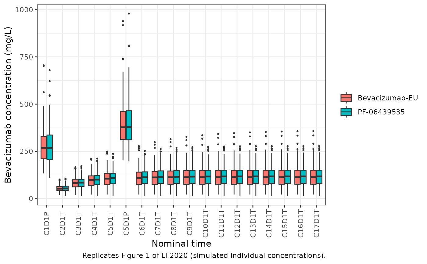
digitised <- data.frame(
  label = c("C1D1P", "C2D1T", "C3D1T", "C4D1T", "C5D1T", "C5D1P", "C8D1T", "C12D1T"),
  published = c(295, 51, 78, 95, 101, 383, 125, 128)
)
fig1_cmp <- nom_sim |>
  dplyr::group_by(label) |>
  dplyr::summarise(simulated = median(Cc), .groups = "drop") |>
  dplyr::inner_join(digitised, by = "label") |>
  dplyr::mutate(pct_diff = 100 * (simulated - published) / published) |>
  dplyr::arrange(match(label, digitised$label))
fig1_cmp |>
  dplyr::rename(
    "Visit" = label,
    "Simulated median (mg/L)" = simulated,
    "Figure 1 median (mg/L)" = published,
    "Difference (%)" = pct_diff
  ) |>
knitr::kable(digits = 1)| Visit | Simulated median (mg/L) | Figure 1 median (mg/L) | Difference (%) |
|---|---|---|---|
| C1D1P | 267.8 | 295 | -9.2 |
| C2D1T | 52.8 | 51 | 3.5 |
| C3D1T | 83.1 | 78 | 6.5 |
| C4D1T | 99.0 | 95 | 4.2 |
| C5D1T | 107.2 | 101 | 6.1 |
| C5D1P | 377.4 | 383 | -1.5 |
| C8D1T | 114.8 | 125 | -8.2 |
| C12D1T | 116.1 | 128 | -9.3 |
The last bound is on eight cohort medians of 400 subjects, which are far more stable across rxode2 builds than per-subject extremes, and it has ample headroom over the digitisation error.
The early visits (Cycles 2-5) agree within about 5%. The Cycle 1 peak is about 10% lower than the observed median, and the late-cycle troughs (Cycles 8 and 12) are about 12% lower than observed. The late-cycle shortfall is consistent with informative dropout: patients who stay on monotherapy through Cycle 12 are those without progression, a subgroup whose bevacizumab clearance tends to be lower. The virtual cohort keeps every patient on treatment. No parameters were adjusted.
Concentration-time profile
sim |>
  # drop the zero pre-dose record, which has no place on a log axis
  dplyr::filter(time != 0) |>
  dplyr::group_by(arm, time) |>
  dplyr::summarise(
    q05 = quantile(Cc, 0.05),
    q50 = median(Cc),
    q95 = quantile(Cc, 0.95),
    .groups = "drop"
  ) |>
  ggplot(aes(time / 24, q50, colour = arm, fill = arm)) +
  geom_ribbon(aes(ymin = q05, ymax = q95), alpha = 0.15, colour = NA) +
  geom_line() +
  scale_y_log10() +
  labs(
    x = "Time (day)",
    y = "Bevacizumab concentration (mg/L)",
    colour = NULL,
    fill = NULL,
    caption = "Median and 90% interval; compare the log-scale VPC in Figure 4a of Li 2020."
  ) +
  theme_bw()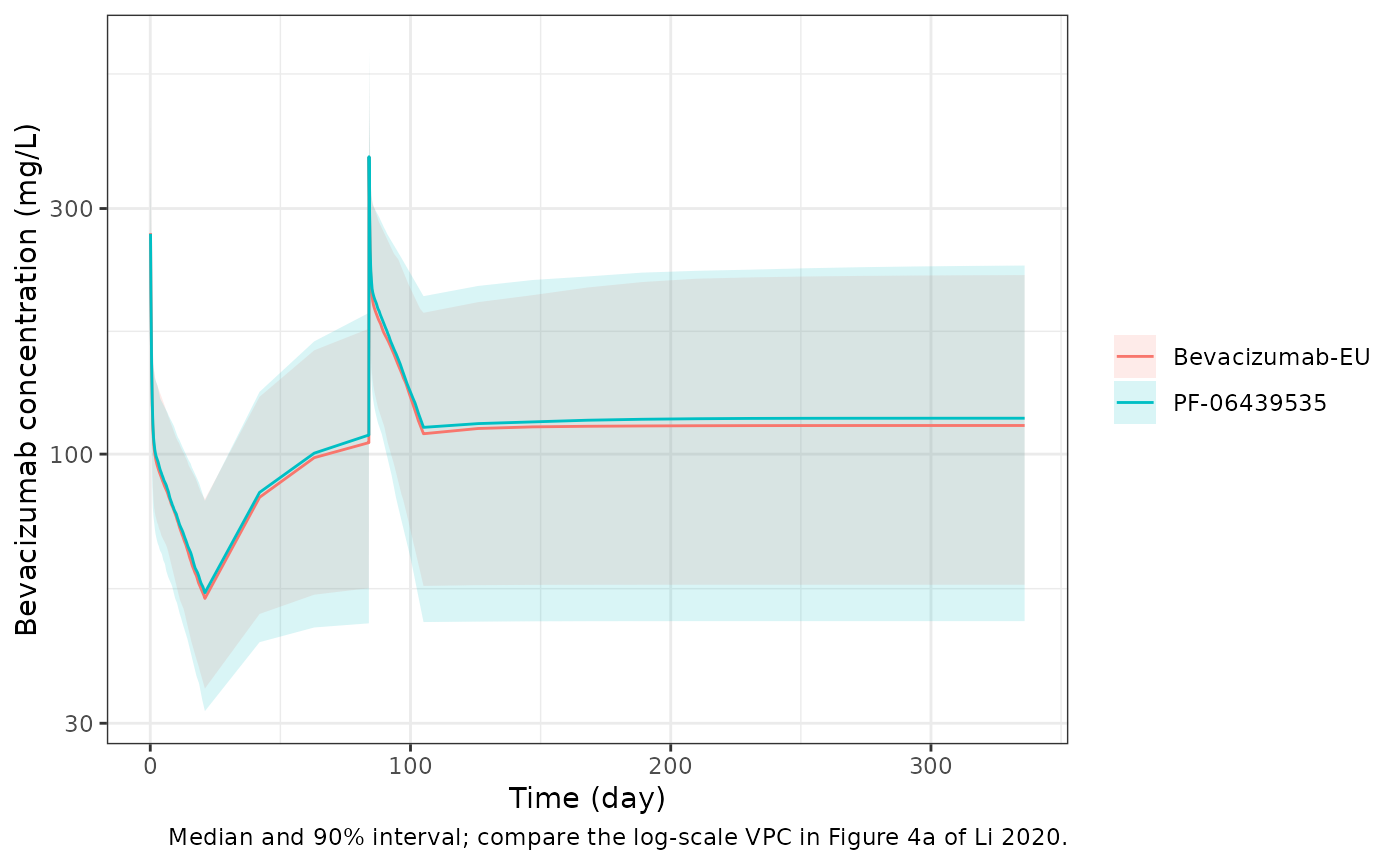
PKNCA validation
NCA over the first dosing interval (Cycle 1) and the fifth (Cycle 5), by arm. Li 2020 did not report NCA parameters, so there is no published NCA table to compare against; the NCA confirms that the two arms differ by the small drug-product effects the model carries (CL 2% and V1 7% higher on PF-06439535), so AUC over a dosing interval should be about 2% lower on PF-06439535.
nca_conc <- sim |>
  dplyr::filter(!is.na(Cc)) |>
  dplyr::filter(time <= tau | (time >= dose_times[5] & time <= dose_times[5] + tau)) |>
  dplyr::select(id, time, Cc, arm) |>
  dplyr::distinct()
nca_dose <- dose_rows |>
  dplyr::filter(cycle %in% c(1, 5)) |>
  dplyr::select(id, time, amt, arm)

conc_obj <- PKNCA::PKNCAconc(nca_conc, Cc ~ time | arm + id)
dose_obj <- PKNCA::PKNCAdose(nca_dose, amt ~ time | arm + id)
intervals <- data.frame(
  start = c(0, dose_times[5]),
  end = c(tau, dose_times[5] + tau),
  cmax = TRUE,
  tmax = TRUE,
  cmin = TRUE,
  auclast = TRUE
)
nca_res <- PKNCA::pk.nca(PKNCA::PKNCAdata(conc_obj, dose_obj, intervals = intervals))
nca_sum <- as.data.frame(nca_res$result) |>
  dplyr::mutate(cycle = ifelse(start == 0, "Cycle 1", "Cycle 5")) |>
  dplyr::group_by(cycle, arm, PPTESTCD) |>
  dplyr::summarise(median = median(PPORRES), .groups = "drop") |>
  tidyr::pivot_wider(names_from = PPTESTCD, values_from = median)
nca_sum |>
  dplyr::rename(
    "Cycle" = cycle,
    "Arm" = arm,
    "Cmax (mg/L)" = cmax,
    "Tmax (h)" = tmax,
    "Cmin (mg/L)" = cmin,
    "AUC0-tau (h*mg/L)" = auclast
  ) |>
knitr::kable(digits = 1)| Cycle | Arm | AUC0-tau (h*mg/L) | Cmax (mg/L) | Cmin (mg/L) | Tmax (h) |
|---|---|---|---|---|---|
| Cycle 1 | Bevacizumab-EU | 39490.9 | 268.7 | 0.0 | 2.5 |
| Cycle 1 | PF-06439535 | 39870.4 | 267.8 | 0.0 | 2.5 |
| Cycle 5 | Bevacizumab-EU | 79246.7 | 377.4 | 105.3 | 1.5 |
| Cycle 5 | PF-06439535 | 80940.8 | 378.2 | 108.9 | 1.5 |
auc_ratio <- nca_sum |>
  dplyr::group_by(cycle) |>
  dplyr::summarise(
    ratio = auclast[arm == "PF-06439535"] / auclast[arm == "Bevacizumab-EU"],
    .groups = "drop"
  )
auc_ratio |>
  dplyr::rename("Cycle" = cycle, "AUC0-tau ratio, PF-06439535 / bevacizumab-EU" = ratio) |>
knitr::kable(digits = 3)| Cycle | AUC0-tau ratio, PF-06439535 / bevacizumab-EU |
|---|---|
| Cycle 1 | 1.010 |
| Cycle 5 | 1.021 |
The Cycle-1 Cmax (about 260-270 mg/L at the end of the 90-min infusion) lies inside the interquartile box of the observed Cycle 1 peaks in Figure 1. The Cycle 1 Cmin is the zero pre-dose concentration at the start of the interval. The Cycle-5 AUC over the dosing interval (about 78,000-80,000 h x mg/L) is approaching the steady-state value dose / CL, which is about 1065 mg / 0.0135 L/h, or roughly 79,000 h x mg/L, for a typical 71-kg patient with the cohort’s sex mix. The arm-to-arm AUC ratios are dominated by the random draw of the two 200-patient cohorts rather than by the 2% drug-product effect, so they are reported rather than asserted.
Assumptions and deviations
-
Residual error scale. The Methods text calls W the
“estimated residual variance”, but Eq. 2 writes ln(Y) = ln(F) + W x eps
with var(eps) = 1, which makes W the standard deviation on the log
scale. The equation is followed:
expSd = 0.284. (A variance of 0.284 would imply an implausible ~57% CV for a mAb ELISA.) - IIV scale. Table 2 reports omega^2 values; sqrt(0.0871) = 29.5% and sqrt(0.117) = 34.2% match the CVs quoted in the Discussion, confirming that the table values are variances.
-
Drug-product and sex encodings. Figure 2 codes sex
Male = 1 / Female = 2 and drug product PF-06439535 = 1 / bevacizumab-EU
= 2; the final-model equations apply the multipliers to males and to
PF-06439535, which is how
SEXF(1 = female) andTRT_PF06439535(1 = PF-06439535) are used. - Supplement. Online Resource Tables S1 (base model) and S2 (covariate search summary) were not needed: the final model is fully specified in the main text and Table 2.
- Virtual cohort. Weight was drawn log-normally around the 71-kg median independently of sex, because the joint weight-by-sex distribution was not published. Infusion durations follow the protocol’s 90/60/30-min schedule, assuming every infusion was tolerated.
- Figure 1 medians were read by eye from the published box plots and carry a reading uncertainty of roughly +/- 10 mg/L.