Delamanid and DM-6705 in children with MDR-TB (Sasaki 2022)
Source:vignettes/articles/Sasaki_2022_delamanid.Rmd
Sasaki_2022_delamanid.RmdModel and source
Sasaki 2022 developed a joint population PK model of delamanid and its major metabolite DM-6705 in children with multidrug-resistant tuberculosis (MDR-TB), used it to find doses that match the adult exposure, and fitted two concentration-QTc (cQT) linear mixed-effects models, one driven by each analyte. The paper contributes three model files, all documented here:
Sasaki_2022_delamanid– the joint delamanid / DM-6705 PK model.Sasaki_2022_delamanid_QTc_dm6705– the cQT model driven by DM-6705, the significant relationship that the paper used for its QTc projections.Sasaki_2022_delamanid_QTc_parent– the cQT model driven by delamanid (slope not significant).Citation: Sasaki T, Svensson EM, Wang X, Wang Y, Hafkin J, Karlsson MO, Mallikaarjun S. Population Pharmacokinetic and Concentration-QTc Analysis of Delamanid in Pediatric Participants with Multidrug-Resistant Tuberculosis. Antimicrob Agents Chemother. 2022;66(2):e01608-21. doi:10.1128/aac.01608-21
Article: https://doi.org/10.1128/aac.01608-21 (open access; PMC8846319)
Supplement: Supplemental File 1 of the article (Tables S1-S5, Figures S1-S7)
mod_pk <- readModelDb("Sasaki_2022_delamanid")
mod_qtc_m <- readModelDb("Sasaki_2022_delamanid_QTc_dm6705")
mod_qtc_p <- readModelDb("Sasaki_2022_delamanid_QTc_parent")

# The DM-6705 states hold delamanid-equivalent mass; the output Cc_dm6705 is
# converted to ng/mL of DM-6705 by the molecular-weight ratio.
mw_ratio <- 465.5 / 534.5
Population
37 children aged 0.67-17 years with MDR-TB, from the phase 1 trial 232 and its phase 2 extension trial 233, conducted in the Philippines (67.6%) and South Africa (32.4%). Participants were enrolled in four age groups (Sasaki 2022 Table 1):
| Group | Age | n | Mean (SD) weight | Formulation | Dose |
|---|---|---|---|---|---|
| 1 | 12-17 years | 7 | 39 (4.59) kg | 50-mg film-coated tablet | 100 mg BID |
| 2 | 6-11 years | 6 | 24.9 (6.79) kg | 50-mg film-coated tablet | 50 mg BID |
| 3 | 3-5 years | 12 | 14.2 (3.2) kg | 25-mg dispersible tablet | 25 mg BID |
| 4 | 0-2 years | 12 | 9.76 (1.83) kg | 5-mg dispersible tablet | 10 mg BID (> 10 kg), 5 mg BID (> 8 to 10 kg), 5 mg QD (5.5 to 8 kg) |
51.4% were female; 67.6% Asian, 5.4% Black and 27% of other race. The final data set contained 634 delamanid and 706 DM-6705 concentrations; the cQT data set contained 354 QT measurements with time-matched concentrations.
Source trace
| Quantity | Value | Source |
|---|---|---|
| Structure: 2-compartment delamanid, 3 transit compartments, 2-compartment DM-6705 | – | Results; Table 2 |
| CL/F, Vc/F, Q/F, Vp/F (33.5 kg) | 17.2 L/h, 346 L, 62.4 L/h, 296 L | Table 2 |
| MAT (film-coated tablet) | 2.73 h | Table 2 |
| CLM/F, VcM/F, QM/F, VpM/F (33.5 kg) | 54.2 L/h, 77.0 L, 425 L/h, 13,150 L | Table 2 |
| Fraction metabolised FM | 1 (fixed) | Results |
| Weight exponents on clearances / volumes, reference weight | 0.75 / 1 (fixed), 33.5 kg | Table 2 and footnote c |
| Dispersible tablet on MAT / F1 | +0.495 / -0.158 (fixed) | Table 2 and footnote a |
| Age on F1 below 2 years | 0.201 per year | Table 2 and footnote c |
| Dose of 50 mg or less on F1 | +0.580 (fixed) | Table 2 and footnote b |
| Age on FM below 6 years | 0.0654 per year | Table 2 and footnote c |
| IIV CL/F, CLM/F, correlation | 16.3%, 33.9%, 0.710 | Table 2 |
| IIV Vp/F, FM | 58.5%, 13.5% | Table 2 |
| IOV F1, MAT | 26.8%, 60.7% | Table 2 |
| Proportional residual error delamanid / DM-6705 | 30.8% / 18.1% | Table 2; Methods |
| Molecular weights delamanid / DM-6705 | 534.5 / 465.5 g/mol | PubChem (not in the paper) |
| cQT equation | DeltaQTc = (theta0 + eta0) + (theta1 + eta1) C + theta2 (QTc0_i - QTc0) | Methods |
| DM-6705 cQT: intercept, slope, baseline effect | 0.923 ms, 0.0613 ms per ng/mL, 0.0309 | Table S5 |
| DM-6705 cQT: var(eta0), var(eta1), residual variance | 59.9, 0.00446, 174 | Table S5 |
| Delamanid cQT: intercept, slope, baseline effect | 1.47 ms, 0.00792 ms per ng/mL, 0.0318 | Table S4 |
| Delamanid cQT: var(eta0), var(eta1), residual variance | 63.5, 0.0000937, 180 | Table S4 |
| Mean baseline QTcB (centering constant) | 421 ms | Derived from Figure S5 and the Discussion (see below) |
Typical-value checks against closed forms
At steady state the dosing-interval AUC of a linear model is
F * Dose / CL for delamanid and
FM * F * Dose / CLM (times the molecular-weight ratio) for
DM-6705. Both sides use the same parameters, so the check is tight and
catches a mis-wired bioavailability, formation term or unit
conversion.
# Build an event table: one dosing row (ii / addl) plus observation rows. With
# two error endpoints every observation row nominates one through dvid.
make_events <- function(id, dose, tau, n_dose, obs_times, wt, age, form, occ = 1) {
  dose_rows <- data.frame(
    id = id, time = 0, amt = dose, evid = 1L, cmt = "depot", dvid = NA_integer_,
    ii = tau, addl = n_dose - 1L
  )
  obs_rows <- data.frame(
    id = id, time = obs_times, amt = 0, evid = 0L, cmt = NA_character_, dvid = 1L,
    ii = 0, addl = 0L
  )
  ev <- dplyr::bind_rows(dose_rows, obs_rows)
  ev$WT <- wt
  ev$AGE <- age
  ev$FORM_DELAMANID_DT <- form
  ev$DOSE_DELAMANID_MG <- dose
  ev$OCC <- occ
  ev
}

trap_auc <- function(t, y) sum(diff(t) * (head(y, -1) + tail(y, -1)) / 2)

groups <- tibble::tribble(
  ~group, ~wt, ~age, ~form, ~dose,
  "Group 1 (12-17 y)", 39.0, 15.3, 0, 100,
  "Group 2 (6-11 y)", 24.9, 9.44, 0, 50,
  "Group 3 (3-5 y)", 14.2, 4.30, 1, 25,
  "Group 4 (0-2 y)", 9.76, 1.68, 1, 10
)
mod_typ <- rxode2::zeroRe(mod_pk)
#> ℹ parameter labels from comments will be replaced by 'label()'
#> Warning: some etas defaulted to non-mu referenced, possible parsing error: etaiov_fdepot_1, etaiov_fdepot_2, etaiov_fdepot_3, etaiov_fdepot_4, etaiov_mtt_1, etaiov_mtt_2, etaiov_mtt_3, etaiov_mtt_4
#> as a work-around try putting the mu-referenced expression on a simple line
#> Warning: some etas defaulted to non-mu referenced, possible parsing error: etaiov_fdepot_1, etaiov_fdepot_2, etaiov_fdepot_3, etaiov_fdepot_4, etaiov_mtt_1, etaiov_mtt_2, etaiov_mtt_3, etaiov_mtt_4
#> as a work-around try putting the mu-referenced expression on a simple line
tau <- 12
n_dose <- 60 * 2 # 60 days BID
t_last <- (n_dose - 1) * tau
obs <- seq(t_last, t_last + tau, by = 0.05)

closed <- lapply(seq_len(nrow(groups)), function(i) {
  g <- groups[i, ]
  ev <- make_events(1, g$dose, tau, n_dose, obs, g$wt, g$age, g$form, occ = 0)
  s <- as.data.frame(rxode2::rxSolve(mod_typ, ev, atol = 1e-10, rtol = 1e-10))
  cl <- 17.2 * (g$wt / 33.5)^0.75
  clm <- 54.2 * (g$wt / 33.5)^0.75
  f1 <- (1 - 0.201 * (2 - g$age) * (g$age < 2)) * (1 - 0.158 * g$form) *
    (1 + 0.580 * (g$dose <= 50))
  fm <- 1 - 0.0654 * (6 - g$age) * (g$age < 6)
  tibble::tibble(
    group = g$group,
    auc_sim = trap_auc(s$time, s$Cc),
    auc_closed = f1 * g$dose * 1000 / cl,
    aucm_sim = trap_auc(s$time, s$Cc_dm6705),
    aucm_closed = fm * f1 * g$dose * 1000 / clm * mw_ratio
  )
}) |> dplyr::bind_rows()
#> ℹ omega/sigma items treated as zero: 'etalcl', 'etalcl_dm6705', 'etalvp', 'etalfm', 'etaiov_fdepot_1', 'etaiov_fdepot_2', 'etaiov_fdepot_3', 'etaiov_fdepot_4', 'etaiov_mtt_1', 'etaiov_mtt_2', 'etaiov_mtt_3', 'etaiov_mtt_4'
#> ℹ omega/sigma items treated as zero: 'etalcl', 'etalcl_dm6705', 'etalvp', 'etalfm', 'etaiov_fdepot_1', 'etaiov_fdepot_2', 'etaiov_fdepot_3', 'etaiov_fdepot_4', 'etaiov_mtt_1', 'etaiov_mtt_2', 'etaiov_mtt_3', 'etaiov_mtt_4'
#> ℹ omega/sigma items treated as zero: 'etalcl', 'etalcl_dm6705', 'etalvp', 'etalfm', 'etaiov_fdepot_1', 'etaiov_fdepot_2', 'etaiov_fdepot_3', 'etaiov_fdepot_4', 'etaiov_mtt_1', 'etaiov_mtt_2', 'etaiov_mtt_3', 'etaiov_mtt_4'
#> ℹ omega/sigma items treated as zero: 'etalcl', 'etalcl_dm6705', 'etalvp', 'etalfm', 'etaiov_fdepot_1', 'etaiov_fdepot_2', 'etaiov_fdepot_3', 'etaiov_fdepot_4', 'etaiov_mtt_1', 'etaiov_mtt_2', 'etaiov_mtt_3', 'etaiov_mtt_4'

knitr::kable(closed, digits = 1, caption = "Steady-state AUC0-12 (ng*h/mL) of the typical child in each age group after 60 days BID: solve vs closed form.")| group | auc_sim | auc_closed | aucm_sim | aucm_closed |
|---|---|---|---|---|
| Group 1 (12-17 y) | 5187.5 | 5187.5 | 1424.1 | 1433.7 |
| Group 2 (6-11 y) | 5737.6 | 5737.6 | 1579.9 | 1585.7 |
| Group 3 (3-5 y) | 3680.8 | 3680.8 | 902.8 | 904.2 |
| Group 4 (0-2 y) | 1825.0 | 1825.0 | 361.6 | 361.9 |
Adjudicating the printed age condition on F1
The Table 2 footnote prints the bioavailability age term as applying “if age is > 2.0 years”. The Table 2 row (“Age on F1: linear slope below 2 yrs”), the Results (“age on F1 only for ages of < 2 years”) and the Discussion (“a linear increase was observed from the ages of 0 to 2 years but not beyond”) all say the opposite, and applied above 2 years the term would grow without bound (F1 = 4.0 at 17 years). The model uses the below-2-years reading. Table 3 settles it: for a 25-kg child aged 10 years given 100 mg of the film-coated tablet once daily, the paper reports a median AUC0-24,ss of 7,320 ng*h/mL.
cl_25 <- 17.2 * (25 / 33.5)^0.75
f1_below2 <- 1 # the age term is off at 10 years
f1_above2 <- 1 - 0.201 * (2 - 10)
adjud <- tibble::tibble(
  reading = c("Age term below 2 years (model)", "Age term above 2 years (as printed)"),
  F1 = c(f1_below2, f1_above2),
  AUC0_24 = c(f1_below2, f1_above2) * 100 * 1000 / cl_25,
  ratio_to_table3 = AUC0_24 / 7320
)
knitr::kable(adjud, digits = 3)| reading | F1 | AUC0_24 | ratio_to_table3 |
|---|---|---|---|
| Age term below 2 years (model) | 1.000 | 7241.027 | 0.989 |
| Age term above 2 years (as printed) | 2.608 | 18884.598 | 2.580 |
Virtual cohort: the trial 232 design
Trial 232 dosed each age group twice daily for 10 days and sampled on days 1-2 and 10-11 and at 72, 120 and 192 h after the last dose (Table S1). The cohort below draws 100 children per age group from the Table 1 mean (SD) of weight and age, redrawing values outside each group’s age range and outside 3-60 kg. Group 4 doses follow the weight rule of Table S1. Occasion 1 covers days 1-9 and occasion 2 day 10 onwards.
rxode2::rxSetSeed(2022)
set.seed(2022)

draw_trunc <- function(n, mean, sd, lo, hi) {
  x <- rnorm(n, mean, sd)
  while (any(bad <- x < lo | x > hi)) x[bad] <- rnorm(sum(bad), mean, sd)
  x
}

grp_spec <- tibble::tribble(
  ~group, ~wt_m, ~wt_sd, ~age_m, ~age_sd, ~age_lo, ~age_hi, ~form,
  "Group 1 (12-17 y)", 39.0, 4.59, 15.3, 1.62, 12, 17.99, 0,
  "Group 2 (6-11 y)", 24.9, 6.79, 9.44, 1.51, 6, 11.99, 0,
  "Group 3 (3-5 y)", 14.2, 3.20, 4.30, 0.988, 3, 5.99, 1,
  "Group 4 (0-2 y)", 9.76, 1.83, 1.68, 0.591, 0.67, 2.99, 1
)
n_per_group <- 100

obs_232 <- sort(unique(c(
  seq(0, 24, by = 1), seq(216, 240, by = 1),
  216 + c(72, 120, 192)
)))

cohort <- lapply(seq_len(nrow(grp_spec)), function(i) {
  g <- grp_spec[i, ]
  tibble::tibble(
    id = (i - 1) * n_per_group + seq_len(n_per_group),
    group = g$group,
    WT = draw_trunc(n_per_group, g$wt_m, g$wt_sd, 3, 60),
    AGE = draw_trunc(n_per_group, g$age_m, g$age_sd, g$age_lo, g$age_hi),
    form = g$form
  )
}) |>
  dplyr::bind_rows() |>
  dplyr::mutate(
    dose = dplyr::case_when(
      group == "Group 1 (12-17 y)" ~ 100,
      group == "Group 2 (6-11 y)" ~ 50,
      group == "Group 3 (3-5 y)" ~ 25,
      WT > 10 ~ 10,
      TRUE ~ 5
    ),
    tau = ifelse(group == "Group 4 (0-2 y)" & WT <= 8, 24, 12)
  )

events_232 <- lapply(seq_len(nrow(cohort)), function(i) {
  p <- cohort[i, ]
  dose_times <- seq(0, 216, by = p$tau)
  ev <- dplyr::bind_rows(
    data.frame(
      id = p$id, time = dose_times, amt = p$dose, evid = 1L,
      cmt = "depot", dvid = NA_integer_
    ),
    data.frame(
      id = p$id, time = obs_232, amt = 0, evid = 0L,
      cmt = NA_character_, dvid = 1L
    )
  )
  ev$WT <- p$WT
  ev$AGE <- p$AGE
  ev$FORM_DELAMANID_DT <- p$form
  ev$DOSE_DELAMANID_MG <- p$dose
  ev$OCC <- ifelse(ev$time < 216, 1L, 2L)
  ev$group <- p$group
  ev
}) |>
  dplyr::bind_rows() |>
  dplyr::arrange(id, time, dplyr::desc(evid))

stopifnot(!anyDuplicated(unique(events_232[, c("id", "time", "evid")])))

sim_232 <- rxode2::rxSolve(mod_pk, events_232, keep = "group") |>
  as.data.frame()
#> ℹ parameter labels from comments will be replaced by 'label()'
#> Warning: some etas defaulted to non-mu referenced, possible parsing error: etaiov_fdepot_1, etaiov_fdepot_2, etaiov_fdepot_3, etaiov_fdepot_4, etaiov_mtt_1, etaiov_mtt_2, etaiov_mtt_3, etaiov_mtt_4
#> as a work-around try putting the mu-referenced expression on a simple line
vpc <- sim_232 |>
  tidyr::pivot_longer(c(Cc, Cc_dm6705), names_to = "analyte", values_to = "conc") |>
  dplyr::mutate(analyte = ifelse(analyte == "Cc", "Delamanid", "DM-6705")) |>
  dplyr::group_by(group, analyte, time) |>
  dplyr::summarise(
    p05 = quantile(conc, 0.05), p50 = median(conc), p95 = quantile(conc, 0.95),
    .groups = "drop"
  )

ggplot(vpc, aes(time / 24, p50)) +
  geom_ribbon(aes(ymin = p05, ymax = p95), fill = "steelblue", alpha = 0.3) +
  geom_line(colour = "steelblue4") +
  facet_grid(analyte ~ group, scales = "free_y") +
  labs(
    x = "Time after first dose (days)", y = "Concentration (ng/mL)",
    caption = "Median and 90% prediction interval, 100 simulated children per group."
  ) +
  theme_bw()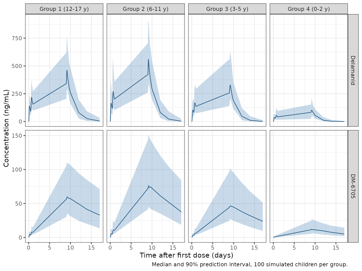
The simulated profiles show the features of the observed data in Figure 1 and the pcVPCs of Figure 3 of Sasaki 2022. Delamanid accumulates over the 10 days of BID dosing. DM-6705 rises steadily over the dosing period and declines only slowly after the last dose, because of its 13,150-L peripheral volume.
PKNCA: day-10 dosing interval
nca_232 <- lapply(c("Cc", "Cc_dm6705"), function(an) {
  conc <- sim_232 |>
    dplyr::filter(time >= 216, time <= 240) |>
    dplyr::select(id, time, group, conc = dplyr::all_of(an)) |>
    dplyr::filter(!is.na(conc)) |>
    dplyr::rename(Cc = conc)
  doses <- events_232 |>
    dplyr::filter(evid == 1, time == 216) |>
    dplyr::select(id, time, amt, group)
  conc_obj <- PKNCA::PKNCAconc(conc, Cc ~ time | group + id)
  dose_obj <- PKNCA::PKNCAdose(doses, amt ~ time | group + id)
  intervals <- data.frame(
    start = 216, end = 228, cmax = TRUE, tmax = TRUE, auclast = TRUE
  )
  res <- PKNCA::pk.nca(PKNCA::PKNCAdata(conc_obj, dose_obj, intervals = intervals))
  as.data.frame(res) |> dplyr::mutate(analyte = an)
}) |> dplyr::bind_rows()

nca_232_summary <- nca_232 |>
  dplyr::group_by(analyte, group, PPTESTCD) |>
  dplyr::summarise(median = median(PPORRES), .groups = "drop") |>
  tidyr::pivot_wider(names_from = PPTESTCD, values_from = median)

nca_232_summary |>
  dplyr::rename(
    "Analyte" = analyte,
    "Group" = group,
    "Cmax (ng/mL)" = cmax,
    "Tmax (h)" = tmax,
    "AUC0-12 (ng*h/mL)" = auclast
  ) |>
knitr::kable(digits = 1, caption = "Median day-10 NCA (216-228 h) by age group. Group 4 includes some once-daily subjects, whose AUC covers half their interval.")| Analyte | Group | AUC0-12 (ng*h/mL) | Cmax (ng/mL) | Tmax (h) |
|---|---|---|---|---|
| Cc | Group 1 (12-17 y) | 4965.0 | 476.7 | 4 |
| Cc | Group 2 (6-11 y) | 5783.9 | 572.9 | 4 |
| Cc | Group 3 (3-5 y) | 3677.3 | 346.5 | 5 |
| Cc | Group 4 (0-2 y) | 1118.8 | 109.2 | 5 |
| Cc_dm6705 | Group 1 (12-17 y) | 701.6 | 59.9 | 5 |
| Cc_dm6705 | Group 2 (6-11 y) | 891.0 | 76.4 | 4 |
| Cc_dm6705 | Group 3 (3-5 y) | 552.6 | 46.9 | 6 |
| Cc_dm6705 | Group 4 (0-2 y) | 140.9 | 12.2 | 6 |
Sasaki 2022 does not tabulate observed NCA for trials 232 and 233, so the quantitative comparison is made against its dose-finding simulations (Table 3) below.
Replicating Table 3: doses matching the adult exposure
Table 3 lists, for each regimen, formulation, age class and weight band, the doses whose median steady-state AUC0-24 falls within 0.80-1.25 of the adult target of 7,500 ng*h/mL. It also gives the median DM-6705 Cmax,ss at the highest of those doses, and the predicted DeltaQTcB at that Cmax. The rows below use the highest listed dose, whose median AUC is the upper value of each printed range. The two rows whose highest dose is the split 50 mg + 25 mg regimen are omitted. The paper resampled age and weight from 266 South African children, which are not published; each row here draws 100 children with weight uniform in the band (50-65 kg for “50 kg or more”, 10-13 kg for the 2 years or younger class) and age uniform over a range matched to the band. Steady state is taken on day 60.
table3 <- tibble::tribble(
  ~row, ~regimen, ~form, ~age_class, ~wt_lo, ~wt_hi, ~dose, ~auc_pub, ~cmaxm_pub, ~dqtc_pub,
  1, "QD", 0, "<=2 y", 10, 20, 40, 7570, 63.4, 3.89,
  2, "QD", 0, ">2 y", 10, 20, 50, 8800, 87.8, 5.38,
  3, "QD", 0, ">2 y", 20, 30, 100, 7320, 82.3, 5.05,
  4, "QD", 1, "<=2 y", 10, 20, 50, 7970, 66.0, 4.05,
  5, "QD", 1, ">2 y", 10, 20, 50, 7410, 73.0, 4.48,
  6, "QD", 1, ">2 y", 20, 30, 100, 6160, 68.6, 4.21,
  7, "BID", 0, "<=2 y", 10, 20, 20, 7570, 61.5, 3.77,
  8, "BID", 0, ">2 y", 10, 20, 25, 8800, 84.9, 5.21,
  9, "BID", 0, ">2 y", 30, 40, 50, 8830, 95.4, 5.85,
  10, "BID", 0, ">2 y", 40, 50, 50, 7440, 78.3, 4.80,
  11, "BID", 0, ">2 y", 50, Inf, 100, 7900, 81.8, 5.02,
  12, "BID", 1, "<=2 y", 10, 20, 25, 7970, 64.4, 3.95,
  13, "BID", 1, ">2 y", 10, 20, 30, 8890, 85.3, 5.23,
  14, "BID", 1, ">2 y", 30, 40, 50, 7580, 81.2, 4.98,
  15, "BID", 1, ">2 y", 40, 50, 100, 7920, 83.1, 5.10,
  16, "BID", 1, ">2 y", 50, Inf, 100, 6650, 68.5, 4.20
) |>
  dplyr::mutate(
    treatment = sprintf(
      "%02d %s %s %s %s-%s kg %g mg", row, regimen,
      ifelse(form == 1, "DT", "FCT"), age_class, wt_lo,
      ifelse(is.finite(wt_hi), wt_hi, "65"), dose
    )
  )
The predicted DeltaQTcB column of Table 3 is the DM-6705 drug effect, slope times Cmax, with the intercept and baseline terms excluded. Evaluating the DM-6705 cQT model at each printed Cmax and subtracting its prediction at zero concentration reproduces the column exactly:
qtc_m_typ <- rxode2::zeroRe(mod_qtc_m)
#> ℹ parameter labels from comments will be replaced by 'label()'
qtc_ev <- data.frame(
  id = 1, time = seq_len(nrow(table3)), evid = 0L,
  CP_DM6705_NGML = table3$cmaxm_pub, QTC_BL = 421
)
qtc_ev0 <- dplyr::mutate(qtc_ev, CP_DM6705_NGML = 0)
drug_effect <- as.data.frame(rxode2::rxSolve(qtc_m_typ, qtc_ev))$QTc -
  as.data.frame(rxode2::rxSolve(qtc_m_typ, qtc_ev0))$QTc
#> ℹ omega/sigma items treated as zero: 'etae0', 'etaslope'
#> ℹ omega/sigma items treated as zero: 'etae0', 'etaslope'

table3$dqtc_model <- drug_effect
stopifnot(all(abs(table3$dqtc_model - table3$dqtc_pub) < 0.01))
rxode2::rxSetSeed(2023)
set.seed(2023)
n_row <- 100
ss_day <- 60

age_range <- function(age_class, wt_lo) {
  if (age_class == "<=2 y") {
    return(c(1, 2))
  }
  switch(as.character(wt_lo),
    "10" = c(2, 6),
    "20" = c(6, 10),
    "30" = c(9, 13),
    "40" = c(11, 15),
    "50" = c(13, 17)
  )
}

events_t3 <- lapply(seq_len(nrow(table3)), function(i) {
  r <- table3[i, ]
  tau <- ifelse(r$regimen == "QD", 24, 12)
  n_dose <- ss_day * 24 / tau
  wt_hi <- ifelse(r$age_class == "<=2 y", 13, ifelse(is.finite(r$wt_hi), r$wt_hi, 65))
  ar <- age_range(r$age_class, r$wt_lo)
  obs <- seq((ss_day - 1) * 24, ss_day * 24, by = 0.5)
  lapply(seq_len(n_row), function(j) {
    ev <- make_events(
      id = (i - 1) * n_row + j, dose = r$dose, tau = tau, n_dose = n_dose,
      obs_times = obs, wt = runif(1, r$wt_lo, wt_hi), age = runif(1, ar[1], ar[2]),
      form = r$form, occ = 1
    )
    ev$treatment <- r$treatment
    ev
  }) |> dplyr::bind_rows()
}) |> dplyr::bind_rows()

stopifnot(!anyDuplicated(unique(events_t3[, c("id", "time", "evid")])))

sim_t3 <- rxode2::rxSolve(mod_pk, events_t3, keep = "treatment") |>
  as.data.frame()
t0 <- (ss_day - 1) * 24
doses_t3 <- events_t3 |>
  dplyr::filter(evid == 1) |>
  dplyr::distinct(id, treatment, amt) |>
  dplyr::mutate(time = t0)

nca_one <- function(col, params) {
  conc <- sim_t3 |>
    dplyr::select(id, time, treatment, Cc = dplyr::all_of(col)) |>
    dplyr::filter(!is.na(Cc))
  intervals <- data.frame(start = t0, end = t0 + 24)
  for (p in params) intervals[[p]] <- TRUE
  PKNCA::pk.nca(PKNCA::PKNCAdata(
    PKNCA::PKNCAconc(conc, Cc ~ time | treatment + id),
    PKNCA::PKNCAdose(doses_t3, amt ~ time | treatment + id),
    intervals = intervals
  ))
}
nca_t3_parent <- nca_one("Cc", "auclast")
nca_t3_metab <- nca_one("Cc_dm6705", "cmax")

sim_t3_long <- dplyr::bind_rows(
  as.data.frame(nca_t3_parent) |> dplyr::filter(PPTESTCD == "auclast"),
  as.data.frame(nca_t3_metab) |> dplyr::filter(PPTESTCD == "cmax")
) |>
  dplyr::select(treatment, PPTESTCD, PPORRES)

reference_t3 <- table3 |>
  dplyr::select(treatment, auclast = auc_pub, cmax = cmaxm_pub)

cmp_t3 <- nlmixr2lib::ncaComparisonTable(
  simulated = sim_t3_long,
  reference = reference_t3,
  by = "treatment",
  units = c(auclast = "ng*h/mL", cmax = "ng/mL"),
  tolerance_pct = 20
)
knitr::kable(
  cmp_t3,
  caption = paste(
    "Sasaki 2022 Table 3 vs simulation: median steady-state delamanid AUC0-24",
    "(AUC0-t) and median steady-state DM-6705 Cmax (Cmax). * differs by more than 20%."
  )
)| NCA parameter | treatment | Reference | Simulated | % diff |
|---|---|---|---|---|
| Cmax (ng/mL) | 01 QD FCT <=2 y 10-20 kg 40 mg | 63.4 | 57.7 | -9.0% |
| Cmax (ng/mL) | 02 QD FCT >2 y 10-20 kg 50 mg | 87.8 | 81.8 | -6.8% |
| Cmax (ng/mL) | 03 QD FCT >2 y 20-30 kg 100 mg | 82.3 | 87.9 | +6.7% |
| Cmax (ng/mL) | 04 QD DT <=2 y 10-20 kg 50 mg | 66 | 65.4 | -0.9% |
| Cmax (ng/mL) | 05 QD DT >2 y 10-20 kg 50 mg | 73 | 68.2 | -6.5% |
| Cmax (ng/mL) | 06 QD DT >2 y 20-30 kg 100 mg | 68.6 | 74.1 | +8.0% |
| Cmax (ng/mL) | 07 BID FCT <=2 y 10-20 kg 20 mg | 61.5 | 64.5 | +4.8% |
| Cmax (ng/mL) | 08 BID FCT >2 y 10-20 kg 25 mg | 84.9 | 97.3 | +14.6% |
| Cmax (ng/mL) | 09 BID FCT >2 y 30-40 kg 50 mg | 95.4 | 108 | +13.1% |
| Cmax (ng/mL) | 10 BID FCT >2 y 40-50 kg 50 mg | 78.3 | 80.6 | +3.0% |
| Cmax (ng/mL) | 11 BID FCT >2 y 50-65 kg 100 mg | 81.8 | 85.8 | +4.9% |
| Cmax (ng/mL) | 12 BID DT <=2 y 10-20 kg 25 mg | 64.4 | 65.4 | +1.5% |
| Cmax (ng/mL) | 13 BID DT >2 y 10-20 kg 30 mg | 85.3 | 84.9 | -0.5% |
| Cmax (ng/mL) | 14 BID DT >2 y 30-40 kg 50 mg | 81.2 | 80.3 | -1.1% |
| Cmax (ng/mL) | 15 BID DT >2 y 40-50 kg 100 mg | 83.1 | 92.9 | +11.7% |
| Cmax (ng/mL) | 16 BID DT >2 y 50-65 kg 100 mg | 68.5 | 78.4 | +14.5% |
| AUClast (ng*h/mL) | 01 QD FCT <=2 y 10-20 kg 40 mg | 7570 | 7240 | -4.4% |
| AUClast (ng*h/mL) | 02 QD FCT >2 y 10-20 kg 50 mg | 8800 | 7720 | -12.3% |
| AUClast (ng*h/mL) | 03 QD FCT >2 y 20-30 kg 100 mg | 7320 | 7400 | +1.1% |
| AUClast (ng*h/mL) | 04 QD DT <=2 y 10-20 kg 50 mg | 7970 | 7730 | -2.9% |
| AUClast (ng*h/mL) | 05 QD DT >2 y 10-20 kg 50 mg | 7410 | 7420 | +0.1% |
| AUClast (ng*h/mL) | 06 QD DT >2 y 20-30 kg 100 mg | 6160 | 6430 | +4.3% |
| AUClast (ng*h/mL) | 07 BID FCT <=2 y 10-20 kg 20 mg | 7570 | 7580 | +0.2% |
| AUClast (ng*h/mL) | 08 BID FCT >2 y 10-20 kg 25 mg | 8800 | 8930 | +1.4% |
| AUClast (ng*h/mL) | 09 BID FCT >2 y 30-40 kg 50 mg | 8830 | 9880 | +11.9% |
| AUClast (ng*h/mL) | 10 BID FCT >2 y 40-50 kg 50 mg | 7440 | 7390 | -0.7% |
| AUClast (ng*h/mL) | 11 BID FCT >2 y 50-65 kg 100 mg | 7900 | 7600 | -3.8% |
| AUClast (ng*h/mL) | 12 BID DT <=2 y 10-20 kg 25 mg | 7970 | 7840 | -1.7% |
| AUClast (ng*h/mL) | 13 BID DT >2 y 10-20 kg 30 mg | 8890 | 8450 | -5.0% |
| AUClast (ng*h/mL) | 14 BID DT >2 y 30-40 kg 50 mg | 7580 | 7190 | -5.1% |
| AUClast (ng*h/mL) | 15 BID DT >2 y 40-50 kg 100 mg | 7920 | 7860 | -0.7% |
| AUClast (ng*h/mL) | 16 BID DT >2 y 50-65 kg 100 mg | 6650 | 6990 | +5.1% |
pct <- sim_t3_long |>
  dplyr::group_by(treatment, PPTESTCD) |>
  dplyr::summarise(sim = median(PPORRES), .groups = "drop") |>
  dplyr::left_join(
    tidyr::pivot_longer(reference_t3, c(auclast, cmax), names_to = "PPTESTCD", values_to = "pub"),
    by = c("treatment", "PPTESTCD")
  ) |>
  dplyr::mutate(pct_diff = 100 * (sim / pub - 1))

pct |>
  dplyr::group_by(PPTESTCD) |>
  dplyr::summarise(
    median_pct_diff = median(pct_diff),
    p90_abs_pct_diff = quantile(abs(pct_diff), 0.9)
  ) |>
knitr::kable(digits = 1)| PPTESTCD | median_pct_diff | p90_abs_pct_diff |
|---|---|---|
| auclast | -0.7 | 8.5 |
| cmax | 3.9 | 13.8 |
# A mis-transcribed clearance, bioavailability term, formation fraction or
# unit moves every row by tens of percent. The envelope is loose because the
# paper's resampled South African demographics are not available and the
# within-band weight and age distributions above are assumptions.
stopifnot(
  abs(median(pct$pct_diff[pct$PPTESTCD == "auclast"])) < 10,
  quantile(abs(pct$pct_diff[pct$PPTESTCD == "auclast"]), 0.9) < 20,
  abs(median(pct$pct_diff[pct$PPTESTCD == "cmax"])) < 12,
  quantile(abs(pct$pct_diff[pct$PPTESTCD == "cmax"]), 0.9) < 25
)
Concentration-QTc models
At the steady-state DM-6705 Cmax values of Table 3 (61.5-95.4 ng/mL), the DM-6705 model gives drug effects of 3.8-5.9 ms (the column reproduced above). The paper concludes that the upper 90% confidence bounds of these effects stay below 10 ms. The delamanid model’s slope is about eight-fold smaller per ng/mL and its confidence interval includes zero.
conc_grid <- seq(0, 150, by = 5)
qtc_p_typ <- rxode2::zeroRe(mod_qtc_p)
#> ℹ parameter labels from comments will be replaced by 'label()'
pred_m <- as.data.frame(rxode2::rxSolve(qtc_m_typ, data.frame(
  id = 1, time = seq_along(conc_grid), evid = 0L,
  CP_DM6705_NGML = conc_grid, QTC_BL = 421
)))
#> ℹ omega/sigma items treated as zero: 'etae0', 'etaslope'
pred_p <- as.data.frame(rxode2::rxSolve(qtc_p_typ, data.frame(
  id = 1, time = seq_along(conc_grid), evid = 0L,
  CP_DELAMANID_NGML = conc_grid, QTC_BL = 421
)))
#> ℹ omega/sigma items treated as zero: 'etae0', 'etaslope'
qtc_df <- dplyr::bind_rows(
  tibble::tibble(conc = conc_grid, dqtc = pred_m$QTc, driver = "DM-6705 (Table S5)"),
  tibble::tibble(conc = conc_grid, dqtc = pred_p$QTc, driver = "Delamanid (Table S4)")
)
ggplot(qtc_df, aes(conc, dqtc, colour = driver)) +
  geom_line() +
  labs(
    x = "Plasma concentration (ng/mL)", y = "Typical DeltaQTcB (ms)",
    colour = NULL, caption = "Typical subject with baseline QTcB equal to the cohort mean (421 ms)."
  ) +
  theme_bw()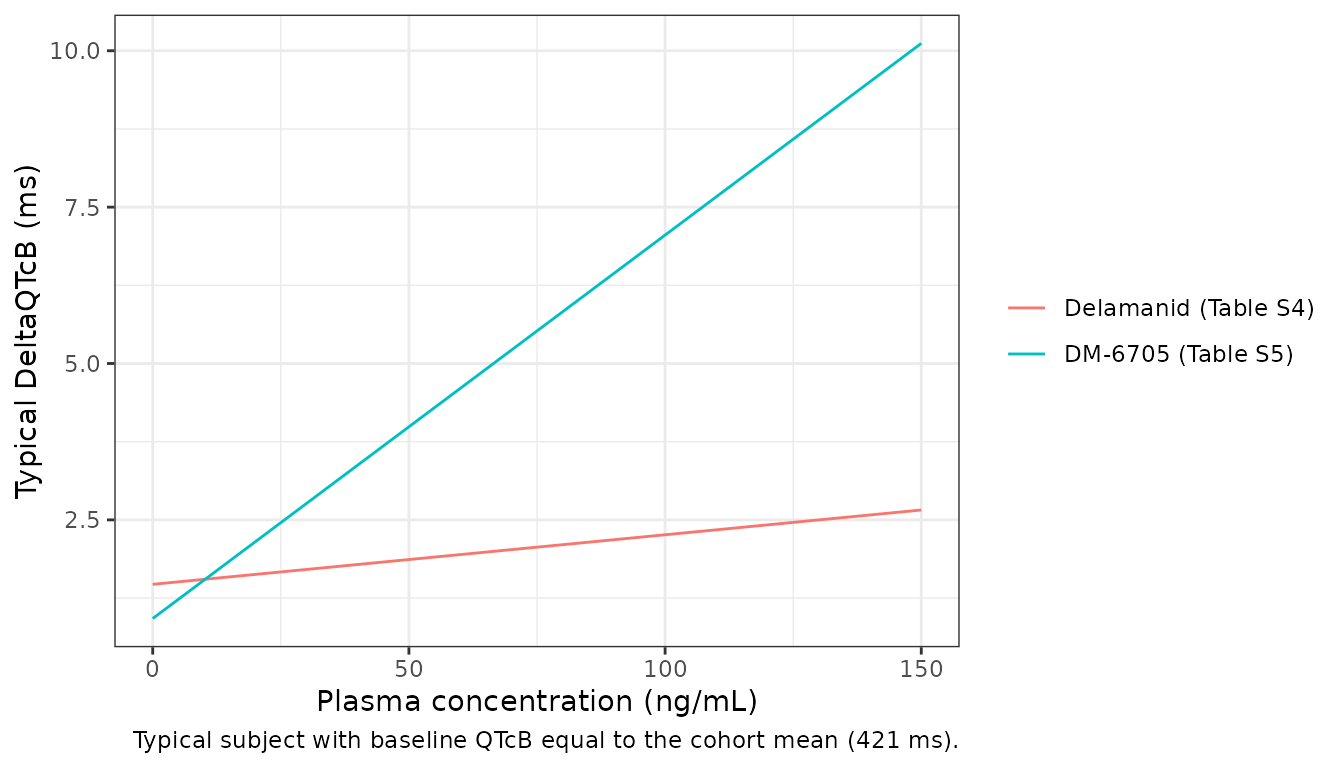
stopifnot(
  abs(diff(range(pred_m$QTc)) - 0.0613 * 150) < 1e-6,
  abs(diff(range(pred_p$QTc)) - 0.00792 * 150) < 1e-6
)
Replicating Figure 4 needs the observed QT data, which are not published. The line above corresponds to its “model fit” line, which is the intercept plus slope term at the mean baseline.
Assumptions and deviations
- Age condition on F1. The Table 2 footnote prints the F1 age term as applying above 2 years. The model applies it below 2 years, as stated in Table 2, the Results and the Discussion, and as Table 3 confirms (see “Adjudicating the printed age condition on F1”).
-
Transit chain. The paper reports “three transit
compartments” and a mean absorption time (MAT) without printing the rate
equation. The model routes the dose through the depot and three transit
compartments into the central compartment, all at rate
ktr = 4 / MAT, so MAT is the mean time through all four first-order steps. Adding transit compartments to a first-order absorption model, as the paper describes, puts them in addition to the absorbing depot. -
Molar units and molecular weights. The model was
fitted to molar concentrations and the paper does not print the
molecular weights. The DM-6705 states hold delamanid-equivalent mass
(formation is mole-for-mole with FM = 1), and
Cc_dm6705is converted to ng/mL with the PubChem molecular weights of delamanid (534.5 g/mol) and DM-6705 (465.5 g/mol). The close agreement with the DM-6705 Cmax column of Table 3 independently supports this conversion. -
Variance scale. Table 2 gives IIV and IOV as CV%;
variances use
omega^2 = log(1 + CV^2). The “71.0” CL/F - CLM/F entry is read as a correlation coefficient. - Residual correlation. The 39.4% correlation between the delamanid and DM-6705 residual errors (Table 2) cannot be expressed in an nlmixr2 model and is omitted. It affects only simulated observations, not individual predictions.
-
Occasions. The paper does not define how occasions
were delimited or how many there were. The model carries four occasions
(
OCC1-4) sharing one variance for F1 and one for MAT; any otherOCCvalue switches the IOV off. -
Dose effect on F1. The +58% bioavailability for
doses of 50 mg or less is applied per dose record through
DOSE_DELAMANID_MG, the dose given at that administration. - cQT centering constant. The cQT equation centers each child’s baseline QTcB on the mean baseline QTcB, QTc0, which the paper does not print. The model uses 421 ms, taken from the baseline QTcB-versus-RR regression of Figure S5 (QTcB = 0.03 RR + 403.167; a least-squares line passes through the mean point) at the mean RR of about 600 ms implied by the Discussion’s baseline heart rate of “approximately 100 bpm”. With baseline coefficients of about 0.03, a 10-ms error in this constant moves the prediction by 0.3 ms.
- Time as a fixed effect. The Methods text says time was a fixed effect in the cQT model, but neither the printed equation nor Tables S4-S5 contain a time term. The models follow the equation and tables.
- Table 3 cohort. The paper’s dose-finding simulations resampled age and weight from two South African pediatric TB studies (n = 266), which are not published. The replication draws weight uniformly within each band and age uniformly over a matched range, and treats day 60 as steady state.
- Screened covariates. BMI and total protein (on CL/F), albumin (on F1) and sex (on Vc/F) were significant in the stepwise search but removed from the final model. No coefficients are reported, so they are recorded as excluded covariates only.