Intra-rectal artesunate / dihydroartemisinin (Simpson 2006)
Source:vignettes/articles/Simpson_2006_artesunate.Rmd
Simpson_2006_artesunate.RmdModel and source
- Citation: Simpson JA, Agbenyega T, Barnes KI, Di Perri G, Folb P, Gomes M, Krishna S, Krudsood S, Looareesuwan S, Mansor S, McIlleron H, Miller R, Molyneux M, Mwenechanya J, Navaratnam V, Nosten F, Olliaro P, Pang L, Ribeiro I, Tembo M, van Vugt M, Ward S, Weerasuriya K, Win K, White NJ. Population pharmacokinetics of artesunate and dihydroartemisinin following intra-rectal dosing of artesunate in malaria patients. PLoS Med. 2006;3(11):e444. doi:10.1371/journal.pmed.0030444
- Description: One-compartment population PK model of dihydroartemisinin (DHA), the principal active metabolite, following a single 10 mg/kg intra-rectal artesunate (ARS) suppository dose in 179 adults and children with moderately severe falciparum malaria pooled from two Phase II and three Phase III studies in Thailand, Ghana, Malawi and South Africa (Simpson 2006). DHA appears by a first-order process whose rate constant (0.2 /h) and lag time (0.14 h) were both fixed because the sparse, erratic data could not identify them; the appearance rate lumps rectal ARS absorption with ARS-to-DHA conversion and is slower than DHA elimination, so the profile is absorption rate limited (flip-flop). Apparent clearance and apparent volume are reported per kilogram: CL/F is a female value plus an additive male increment, and V/F is an affine function of body weight normalised to 70 kg. Artesunate itself could not be modelled - the ARS concentration-time data were too erratic to support a compartmental fit - so no parent PK is included here.
- Article: https://doi.org/10.1371/journal.pmed.0030444
- Open-access full text: https://www.ncbi.nlm.nih.gov/pmc/articles/PMC1664603/
Simpson 2006 pooled five trials of a single intra-rectal artesunate (ARS) suppository dose, nominally 10 mg/kg, given to adults and children with moderately severe Plasmodium falciparum malaria who could not take oral medication. The paper contains one fitted pharmacokinetic model, for the active metabolite dihydroartemisinin (DHA). Artesunate itself was not modelled: “A clear pharmacokinetic profile is difficult to discern, precluding formal pharmacokinetic modelling” (Results, Artesunate Pharmacokinetics), a point the Discussion repeats (“it was not possible to derive the pharmacokinetics of ARS”). This vignette therefore validates the DHA model only.
Population
179 patients from two Phase II studies with intensive sampling (12 adults in Bangkok, Thailand; 11 children in Ghana) and three Phase III studies with sparse or fixed sampling (44 children in Mae-Sot, Thailand; 86 children in Malawi; 26 adults in South Africa). Ages spanned 11 months to 58 years and body weights 7.6 to 86 kg (Table 1 and Table 2). Every patient received the nearest approximation to a single 10 mg/kg intra-rectal artesunate dose using 50 mg and 200 mg suppositories; per-site mean actual doses were 9.2 to 11.0 mg/kg (Table 2). All patients had asexual parasitaemia between 0.1% and 27% and were unable to tolerate oral medication, but had no clinical or laboratory features of severe malaria.
424 DHA concentrations from 164 patients entered the DHA model (three outliers above 6,000 ng/mL were excluded); 164 of the 179 patients obtained posterior individual estimates of CL/F and V/F. Concentrations below the limit of quantification (50 ng/mL, or 20 ng/mL at Mae-Sot) and above the assay range (3,200 ng/mL) were retained rather than censored, because “a large number of these levels are present and exclusion would reduce the power of the statistical modelling” (Methods).
The same information is available programmatically via the model’s
population metadata:
pop <- rxode2::rxode(readModelDb("Simpson_2006_artesunate"))$population
str(pop, max.level = 1)
#> List of 13
#>  $ species       : chr "human"
#>  $ n_subjects    : int 179
#>  $ n_studies     : int 5
#>  $ n_subjects_pk : chr "164 of 179 patients had posterior individual estimates of CL/F and V/F; 424 DHA concentrations from 164 patient"| __truncated__
#>  $ age_range     : chr "11 months to 58 years (Table 1: Bangkok 16-50 y, Ghana 2-7 y, Mae-Sot 11 months-15 y, Malawi 16 months-10 y, So"| __truncated__
#>  $ weight_range  : chr "7.6 to 86 kg (Table 2 per-site ranges; site mean weights 14.2 to 61.9 kg)"
#>  $ sex_female_pct: num 46
#>  $ race_ethnicity: chr "Not reported by race; sites were Thai (Bangkok, Mae-Sot) and African (Ghana, Malawi, South Africa)"
#>  $ disease_state : chr "Moderately severe Plasmodium falciparum malaria (asexual parasite density 0.1-27%) in patients unable to tolera"| __truncated__
#>  $ dose_range    : chr "Single intra-rectal artesunate dose targeting 10 mg/kg (50 mg and 200 mg suppositories, Mepha); per-site mean a"| __truncated__
#>  $ sampling      : chr "Phase II intensive (8 samples over 12 h in Ghana, 9 samples over 12 h in Bangkok); Phase III fixed 5 samples ov"| __truncated__
#>  $ regions       : chr "Thailand (Bangkok, Mae-Sot), Ghana, Malawi, South Africa"
#>  $ notes         : chr "Demographics from Simpson 2006 Tables 1 and 2; baseline laboratory data in Table 3. sex_female_pct is derived a"| __truncated__
Source trace
The per-parameter origin is recorded as an in-file comment next to
each ini() entry in
inst/modeldb/specificDrugs/Simpson_2006_artesunate.R. The
table below collects them in one place for review. Simpson 2006 has no
supplement; Table 5 and the equation image are published only as figures
in the PLoS Medicine article, so every value below was read from the
rendered Table 5 image (pmed.0030444.t005.jpg) in the PMC
supplementary-files bundle.
| Equation / parameter | Value | Source location |
|---|---|---|
lka |
log(0.2), fixed |
Table 5, row “k_a (/h) - fixed” = 0.2; Results DHA Pharmacokinetics “appearance rate was fixed at 0.2/h” |
ltlag |
log(0.14), fixed |
Table 5, row “Lag time (h) - fixed” = 0.14; Results DHA Pharmacokinetics “lag time at 0.14 h” |
lcl |
log(2.03) |
Table 5, row “CL/F (l/kg/h) for a: Female” = 2.03 |
e_male_cl |
1.14 |
Table 5, row “Increase in CL/F (l/kg/h) for a male” = 1.14 (SE 0.40); Abstract 95% CI 0.36 to 1.92 |
lvc |
log(0.57) |
Table 5, row “Intercept” = 0.57 (SE 1.68) |
e_wt_vc |
5.77 |
Table 5, row “Increase in V/F per unit (l/70 kg)” = 5.77 (SE 0.55) |
etalcl |
0.62^2 |
Table 5, row “Inter-individual variability for CL/F” = 62 %CV; Methods: %CV “approximated by the square root of the variance estimate” |
etalvc |
0.75^2 |
Table 5, row “Inter-individual variability for V/F” = 75 %CV, same %CV definition |
expSd |
0.93 |
Table 5, row “Intra-individual variability” = 93 %CV; Results: “a lognormal residual error model for all the data” |
| eta correlation set to zero | n/a | Results DHA Pharmacokinetics: “The data did not support a full variance-covariance matrix for the random effects of CL/F and V/F” |
CL/F = 2.03 + 1.14 * male |
n/a | Table 5 prints both endpoints (male 3.17, female 2.03) and 2.03 + 1.14 = 3.17 |
V/F = 0.57 + 5.77 * (WT/70) |
n/a | Table 5 intercept + slope; reproduces the four printed typical values (15 kg 1.81, 30 kg 3.04, 60 kg 5.52, 70 kg 6.34 L/kg) |
d/dt(depot) = -ka * depot;
d/dt(central) = ka * depot - kel * central;
alag(depot) = tlag
|
n/a | Results DHA Pharmacokinetics: “A one-compartment model with first-order appearance and elimination kinetics including lag time best fits the data” |
| dose = administered artesunate amount, no molar correction | n/a | Methods Population Pharmacokinetic Modelling: “It was assumed that ARS was converted completely to DHA … The exact dose (mg/kg) administered was used in the modelling” |
| Individual parameter = typical * exp(eta) | n/a | Equation 1 of the paper,
(CL/F)_i = (CL/F) * exp(eta_i)
|
Note on the parameterisation: CL/F and V/F are published per
kilogram of body weight, and both covariate effects are
additive on that per-kilogram scale. The Methods
describe weight as entering “using allometric scaling, i.e. (weight/70)
for V/F and (weight/70)^0.75 for CL/F”, but the final model in Table 5
keeps only the linear (WT/70) term on V/F, added to an
intercept, and retains no weight effect at all on CL/F (“No correlation
was observed between eta_CL/F and body weight”, Results). The affine
form is what reproduces the four published typical volumes exactly, so
it is what the model file encodes; the check below is the evidence.
mod <- readModelDb("Simpson_2006_artesunate")
ui <- rxode2::rxode(mod)
ui$iniDf |>
  dplyr::filter(!is.na(ntheta)) |>
  dplyr::select(name, est, fix, label) |>
  dplyr::rename(
    "Parameter" = name, "Estimate (transformed scale)" = est,
    "Fixed" = fix, "Label" = label
  ) |>
knitr::kable(digits = 4, caption = "ini() fixed effects as packaged.")| Parameter | Estimate (transformed scale) | Fixed | Label |
|---|---|---|---|
| lka | -1.6094 | TRUE | First-order appearance rate constant of DHA (1/h) |
| ltlag | -1.9661 | TRUE | Appearance lag time (h) |
| lcl | 0.7080 | FALSE | Apparent DHA clearance for a female (L/kg/h) |
| e_male_cl | 1.1400 | FALSE | Additive increase in apparent DHA clearance for a male (CL/F, L/kg/h; applied as (1 - SEXF)) |
| lvc | -0.5621 | FALSE | Intercept of the apparent DHA volume of distribution (L/kg) |
| e_wt_vc | 5.7700 | FALSE | Increase in apparent DHA volume of distribution per unit of WT/70 (L/kg) |
| expSd | 0.9300 | FALSE | Log-normal residual SD for DHA plasma concentration (SD on the log scale) |
Check 1: typical values reproduce Table 5 exactly
This is a deterministic check on the transcription: with the random effects zeroed, the model must return the sex-specific CL/F and the four weight-specific V/F values printed in Table 5. Both sides use the same parameters, so the tolerance is numerical, not statistical.
table5 <- tidyr::expand_grid(
  WT = c(15, 30, 60, 70),
  SEXF = c(0, 1)
) |>
  dplyr::mutate(id = dplyr::row_number())

ev_typ <- dplyr::bind_rows(
  table5 |> dplyr::mutate(time = 0, amt = 10 * WT, evid = 1L, cmt = "depot"),
  tidyr::crossing(table5, time = c(0.5, 1, 2)) |>
    dplyr::mutate(amt = NA_real_, evid = 0L, cmt = "central")
) |>
  dplyr::arrange(id, time, dplyr::desc(evid))

mod_typ <- rxode2::zeroRe(ui)
sim_typ <- rxode2::rxSolve(
  mod_typ, events = ev_typ, keep = c("WT", "SEXF"), returnType = "data.frame"
)
#> ℹ omega/sigma items treated as zero: 'etalcl', 'etalvc'
#> Warning: multi-subject simulation without without 'omega'

typ <- sim_typ |>
  dplyr::group_by(id) |>
  dplyr::summarise(
    WT = dplyr::first(WT), SEXF = dplyr::first(SEXF),
    clkg = dplyr::first(clkg), vckg = dplyr::first(vckg),
    .groups = "drop"
  ) |>
  dplyr::mutate(
    Sex = ifelse(SEXF == 1, "Female", "Male"),
    published_cl = ifelse(SEXF == 1, 2.03, 3.17),
    published_vc = 0.57 + 5.77 * WT / 70
  )

# Table 5 prints V/F only for these four weights; the printed values are
# 1.81 / 3.04 / 5.52 / 6.34 L/kg.
printed_vc <- c(`15` = 1.81, `30` = 3.04, `60` = 5.52, `70` = 6.34)

typ |>
  dplyr::transmute(
    `Body weight (kg)` = WT,
    Sex = Sex,
    `CL/F model (L/kg/h)` = clkg,
    `CL/F Table 5 (L/kg/h)` = published_cl,
    `V/F model (L/kg)` = vckg,
    `V/F Table 5 (L/kg)` = printed_vc[as.character(WT)]
  ) |>
  knitr::kable(
    digits = 3,
    caption = "Model typical values against the printed values in Simpson 2006 Table 5."
)| Body weight (kg) | Sex | CL/F model (L/kg/h) | CL/F Table 5 (L/kg/h) | V/F model (L/kg) | V/F Table 5 (L/kg) |
|---|---|---|---|---|---|
| 15 | Male | 3.17 | 3.17 | 1.806 | 1.81 |
| 15 | Female | 2.03 | 2.03 | 1.806 | 1.81 |
| 30 | Male | 3.17 | 3.17 | 3.043 | 3.04 |
| 30 | Female | 2.03 | 2.03 | 3.043 | 3.04 |
| 60 | Male | 3.17 | 3.17 | 5.516 | 5.52 |
| 60 | Female | 2.03 | 2.03 | 5.516 | 5.52 |
| 70 | Male | 3.17 | 3.17 | 6.340 | 6.34 |
| 70 | Female | 2.03 | 2.03 | 6.340 | 6.34 |
stopifnot(
  # Deterministic: same parameters on both sides, so machine precision applies.
  max(abs(typ$clkg - typ$published_cl)) < 1e-10,
  # Table 5 prints V/F to 3 significant figures, so compare at that resolution.
  max(abs(typ$vckg - printed_vc[as.character(typ$WT)])) < 0.005
)
Both sex-specific clearances and all four printed volumes are
reproduced. The affine 0.57 + 5.77 * (WT/70) reading of
Table 5 is therefore correct; a power (allometric) reading of the same
two numbers is not, and would miss every printed volume.
Check 2: the base model, its 43-minute half-life, and Figure 2
Before the covariates were added, Simpson 2006 reports a
covariate-free base model with CL/F = 2.64 L/kg/h and V/F = 2.75 L/kg,
“corresponding to an elimination half-life of 43 min” (Abstract and
Results). Figure 2’s solid line is the population prediction from that
base model for a 10 mg/kg dose. The base model is not what the package
ships (the package ships the final model of Table 5), but it is
recoverable by re-ini()-ing the covariate terms away, and
reproducing it is a direct check on the structural equations.
mod_base <- ui |>
  rxode2::ini(
    lcl = log(2.64),      # Abstract / Results: base-model CL/F = 2.64 L/kg/h
    e_male_cl = 0,        # base model has no sex effect
    lvc = log(2.75),      # Abstract / Results: base-model V/F = 2.75 L/kg
    e_wt_vc = 0           # base model has no weight effect
  ) |>
  rxode2::zeroRe()
#> ℹ change initial estimate of `lcl` to `0.970778917158225`
#> ℹ change initial estimate of `e_male_cl` to `0`
#> ℹ change initial estimate of `lvc` to `1.01160091167848`
#> ℹ change initial estimate of `e_wt_vc` to `0`

# Published elimination half-life: log(2) * V/F / (CL/F).
thalf_base_min <- log(2) * 2.75 / 2.64 * 60
thalf_base_min
#> [1] 43.3217

stopifnot(abs(thalf_base_min - 43) < 1)
The base-model elimination half-life is 43.3 min, matching the published 43 min.
tgrid <- sort(unique(c(seq(0, 6, by = 0.02), seq(6, 24, by = 0.1))))
ev_base <- dplyr::bind_rows(
  tibble::tibble(
    id = 1L, time = 0, amt = 10 * 70, evid = 1L, cmt = "depot",
    WT = 70, SEXF = 1
  ),
  tibble::tibble(
    id = 1L, time = tgrid, amt = NA_real_, evid = 0L, cmt = "central",
    WT = 70, SEXF = 1
  )
) |>
  dplyr::arrange(time, dplyr::desc(evid))

# Tight tolerances: the closed-form gate below asserts 1e-8 relative
# agreement, and the default rtol = 1e-6 leaves about 2e-7 when the model is
# integrated numerically.
sim_base <- rxode2::rxSolve(
  mod_base, events = ev_base, returnType = "data.frame",
  rtol = 1e-10, atol = 1e-12
)
#> ℹ omega/sigma items treated as zero: 'etalcl', 'etalvc'
if (is.null(sim_base$id)) sim_base$id <- 1L

# Closed form for a one-compartment model with first-order input and lag:
#   C(t) = (D/V) * ka/(ka - kel) * (exp(-kel*(t-tlag)) - exp(-ka*(t-tlag)))
D_over_V <- 10 / 2.75   # mg/kg / (L/kg) = mg/L, weight cancels
kel_base <- 2.64 / 2.75
ka_base <- 0.2
tlag_base <- 0.14
sim_base <- sim_base |>
  dplyr::mutate(
    tprime = pmax(time - tlag_base, 0),
    closed_form = ifelse(
      time <= tlag_base, 0,
      D_over_V * ka_base / (ka_base - kel_base) *
        (exp(-kel_base * tprime) - exp(-ka_base * tprime))
    )
  )

cf <- sim_base |> dplyr::filter(closed_form > 1e-8)
stopifnot(max(abs(cf$Cc - cf$closed_form) / cf$closed_form) < 1e-8)

ggplot(sim_base |> dplyr::filter(time > 0), aes(time, Cc * 1000)) +
  geom_line(linewidth = 1) +
  geom_line(aes(y = closed_form * 1000), linetype = "dashed", colour = "firebrick") +
  scale_y_log10(limits = c(10, 10000)) +
  scale_x_continuous(breaks = seq(0, 24, by = 4), limits = c(0, 24)) +
  labs(
    x = "Time post dose (h)", y = "DHA concentration (ng/mL)",
    title = "Figure 2 - population-predicted DHA profile, 10 mg/kg",
    caption = "Replicates the solid line of Figure 2 of Simpson 2006."
  ) +
  theme_bw()
#> Warning in scale_y_log10(limits = c(10, 10000)): log-10 transformation introduced infinite values.
#> log-10 transformation introduced infinite values.
#> Warning: Removed 11 rows containing missing values or values outside the scale range
#> (`geom_line()`).
#> Removed 11 rows containing missing values or values outside the scale range
#> (`geom_line()`).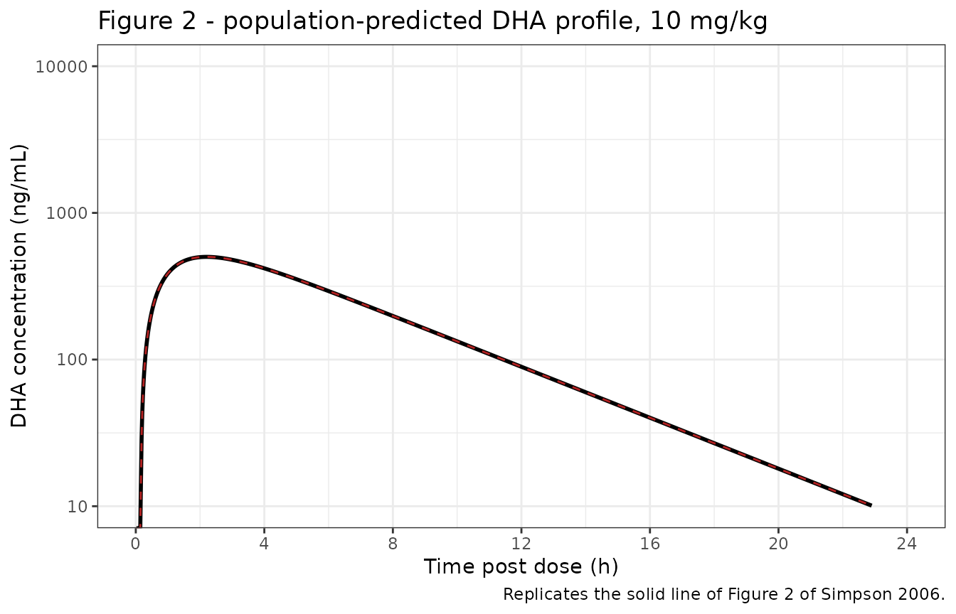
Replicates the population-predicted line of Figure 2 of Simpson 2006 (DHA, 10 mg/kg intra-rectal artesunate). The dashed line is the closed-form solution of the same one-compartment model.
The rxode2 solve and the closed form agree to machine precision, and the curve matches Figure 2: it peaks near 500 ng/mL and falls to roughly 15 ng/mL by 21 h.
The terminal slope is the discriminating feature. Because the fixed
appearance rate (0.2 /h) is much slower than the base-model elimination
rate constant (0.96 /h), the profile is absorption rate limited
(flip-flop) and the terminal log-linear slope should equal
ka, not kel – which is precisely what the
Discussion claims: “The fixed value of the appearance rate constant was
slower than the estimated elimination rate constant, suggesting that the
ARS rectal capsules are absorption rate limited.”
tail_fit <- sim_base |> dplyr::filter(time >= 12, time <= 24, Cc > 0)
slope <- stats::coef(stats::lm(log(Cc) ~ time, data = tail_fit))[["time"]]
c(terminal_slope = slope, ka = 0.2, kel = 2.64 / 2.75)
#> terminal_slope             ka            kel
#>     -0.1999947      0.2000000      0.9600000

# Deterministic (typical-value solve, no cohort draw): the terminal slope must
# be the fixed appearance rate, not the elimination rate constant.
stopifnot(abs(slope + 0.2) < 0.005)
Virtual cohort
Original observed data are not publicly available. The cohort below reproduces the five study sites of Table 1 and Table 2: 100 virtual patients per site (below the 200-per-arm cap), body weight drawn from a normal distribution truncated to the published per-site range, sex drawn from the published per-site percent-male, and the dose set to the published per-site mean in mg/kg.
# rxSetSeed() fixes rxode2's stream for a given thread count only; set.seed()
# fixes R's RNG for the covariate draws. Neither makes the cohort identical
# across machines with different thread counts, so every assertion below is
# written on centres and robust quantiles rather than on extremes.
rxode2::rxSetSeed(20061101)
set.seed(20061101)

sites <- tibble::tribble(
  ~site,          ~n,   ~wt_mean, ~wt_sd, ~wt_lo, ~wt_hi, ~pct_male, ~dose_mgkg,
  "Bangkok",      100L, 48.00,    7.06,   40.0,   60.0,   42,        10.0,
  "Ghana",        100L, 14.91,    3.61,   11.0,   23.0,   55,         9.2,
  "Mae-Sot",      100L, 19.13,    9.30,    9.0,   41.5,   39,        10.3,
  "Malawi",       100L, 14.23,    3.73,    7.6,   25.4,   62,        11.0,
  "South Africa", 100L, 61.92,   10.00,   40.0,   86.0,   58,         9.9
)

rtruncnorm <- function(n, mean, sd, lo, hi) {
  x <- stats::rnorm(n, mean, sd)
  bad <- x < lo | x > hi
  while (any(bad)) {
    x[bad] <- stats::rnorm(sum(bad), mean, sd)
    bad <- x < lo | x > hi
  }
  x
}

obs_times <- sort(unique(c(seq(0, 6, by = 0.1), seq(6.25, 24, by = 0.25))))

make_cohort <- function(i) {
  s <- sites[i, ]
  subj <- tibble::tibble(
    id = (i - 1L) * 1000L + seq_len(s$n),
    site = s$site,
    WT = rtruncnorm(s$n, s$wt_mean, s$wt_sd, s$wt_lo, s$wt_hi),
    SEXF = stats::rbinom(s$n, 1, 1 - s$pct_male / 100)
  ) |>
    dplyr::mutate(amt_mg = s$dose_mgkg * WT)
  dplyr::bind_rows(
    subj |> dplyr::mutate(time = 0, amt = amt_mg, evid = 1L, cmt = "depot"),
    tidyr::crossing(subj, time = obs_times) |>
      dplyr::mutate(amt = NA_real_, evid = 0L, cmt = "central")
  ) |>
    dplyr::arrange(id, time, dplyr::desc(evid))
}

events <- dplyr::bind_rows(lapply(seq_len(nrow(sites)), make_cohort))
stopifnot(!anyDuplicated(unique(events[, c("id", "time", "evid")])))

events |>
  dplyr::filter(evid == 1L) |>
  dplyr::group_by(site) |>
  dplyr::summarise(
    n = dplyr::n(),
    `Mean WT (kg)` = mean(WT),
    `Percent female` = 100 * mean(SEXF),
    `Mean dose (mg/kg)` = mean(amt_mg / WT),
    .groups = "drop"
  ) |>
  dplyr::rename("Study site" = site, "N" = n) |>
knitr::kable(digits = 1, caption = "Virtual cohort against Simpson 2006 Table 2.")| Study site | N | Mean WT (kg) | Percent female | Mean dose (mg/kg) |
|---|---|---|---|---|
| Bangkok | 100 | 48.4 | 57 | 10.0 |
| Ghana | 100 | 16.0 | 42 | 9.2 |
| Mae-Sot | 100 | 22.4 | 69 | 10.3 |
| Malawi | 100 | 15.3 | 35 | 11.0 |
| South Africa | 100 | 62.2 | 43 | 9.9 |
Simulation
sim <- rxode2::rxSolve(
  mod, events = events,
  keep = c("site", "WT", "SEXF", "amt_mg"),
  returnType = "data.frame"
)
stopifnot(all(sim$Cc >= 0), !anyNA(sim$Cc))
vpc <- sim |>
  dplyr::filter(time > 0) |>
  dplyr::group_by(site, time) |>
  dplyr::summarise(
    Q05 = stats::quantile(Cc, 0.05),
    Q50 = stats::quantile(Cc, 0.50),
    Q95 = stats::quantile(Cc, 0.95),
    .groups = "drop"
  )

ggplot(vpc, aes(time, Q50 * 1000)) +
  geom_ribbon(aes(ymin = Q05 * 1000, ymax = Q95 * 1000), alpha = 0.25) +
  geom_line(linewidth = 0.8) +
  geom_line(
    data = sim_base |> dplyr::filter(time > 0) |> dplyr::select(time, Cc),
    aes(time, Cc * 1000), colour = "firebrick", linetype = "dashed"
  ) +
  facet_wrap(~site) +
  scale_y_log10() +
  scale_x_continuous(breaks = seq(0, 24, by = 8)) +
  labs(
    x = "Time post dose (h)", y = "DHA concentration (ng/mL)",
    caption = paste(
      "Median with 5th-95th percentile band per site.",
      "Dashed red line: base-model population prediction (Figure 2)."
    )
  ) +
  theme_bw()
#> Warning in scale_y_log10(): log-10 transformation introduced infinite values.
#> log-10 transformation introduced infinite values.
#> log-10 transformation introduced infinite values.
#> log-10 transformation introduced infinite values.
#> log-10 transformation introduced infinite values.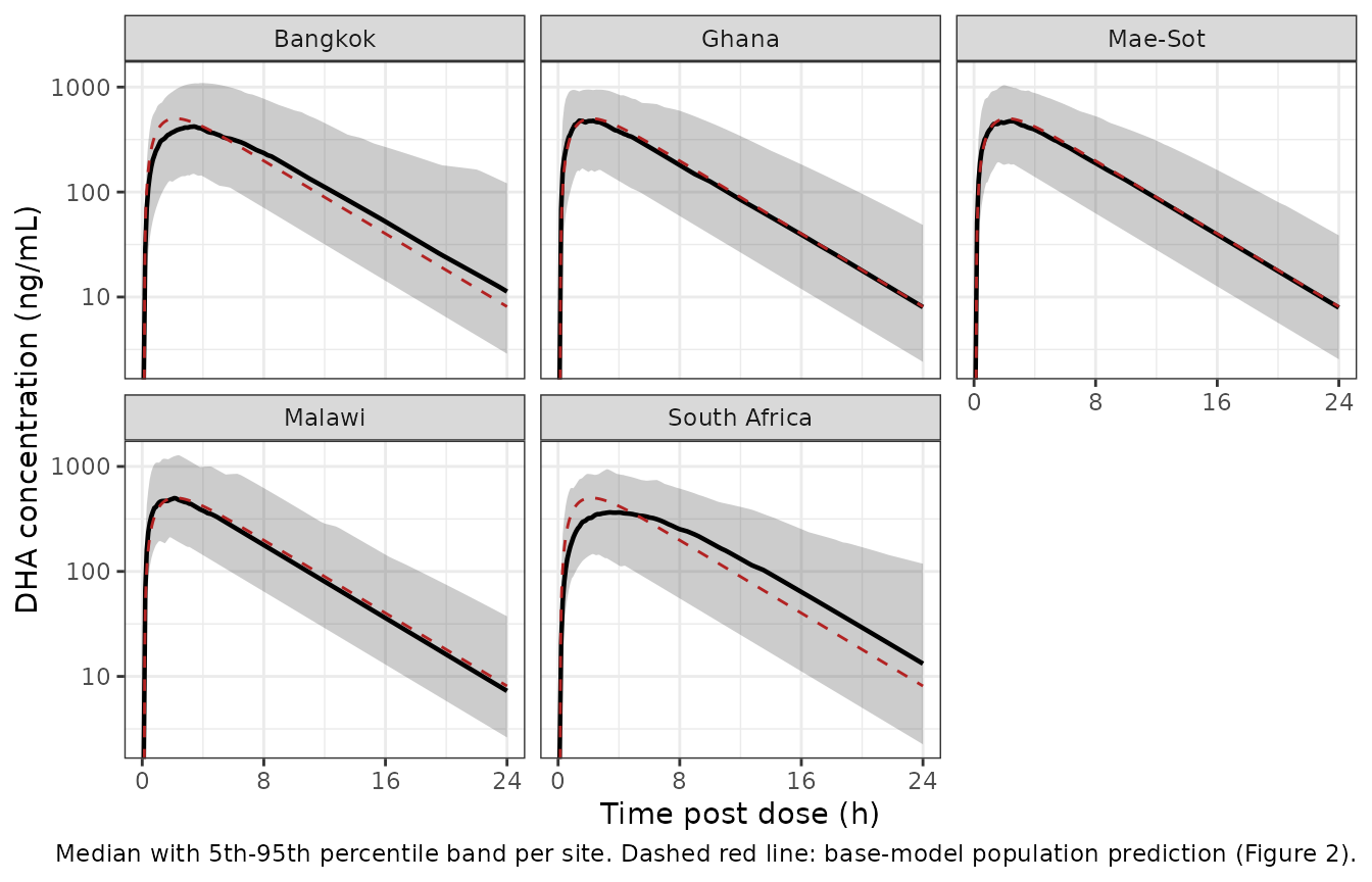
Simulated DHA concentration-time percentiles by study site, with the base-model population prediction of Figure 2 overlaid.
PKNCA validation
sim_nca <- sim |>
  dplyr::filter(!is.na(Cc)) |>
  dplyr::select(id, time, Cc, site)

# Guarantee a time = 0 record per subject; for extravascular dosing Cc = 0 at
# time zero is the correct pre-dose value.
sim_nca <- dplyr::bind_rows(
  sim_nca,
  sim_nca |> dplyr::distinct(id, site) |> dplyr::mutate(time = 0, Cc = 0)
) |>
  dplyr::distinct(id, site, time, .keep_all = TRUE) |>
  dplyr::arrange(id, site, time)

conc_obj <- PKNCA::PKNCAconc(sim_nca, Cc ~ time | site + id)

dose_df <- events |>
  dplyr::filter(evid == 1L) |>
  dplyr::select(id, time, amt, site)
dose_obj <- PKNCA::PKNCAdose(dose_df, amt ~ time | site + id)

# Two intervals: 0-6 h reproduces the exposure metric Simpson 2006 used for its
# pharmacodynamic analysis (AUC0-6h, Figure 5); 0-Inf supports the Dose/CL
# identity check and the terminal half-life.
intervals <- data.frame(
  start      = 0,
  end        = c(6, Inf),
  cmax       = c(TRUE,  FALSE),
  tmax       = c(TRUE,  FALSE),
  auclast    = c(TRUE,  FALSE),
  aucinf.obs = c(FALSE, TRUE),
  half.life  = c(FALSE, TRUE)
)

nca_res <- PKNCA::pk.nca(PKNCA::PKNCAdata(conc_obj, dose_obj, intervals = intervals))

nca_long <- as.data.frame(nca_res) |> dplyr::filter(!is.na(PPORRES))
nca_06 <- nca_long |>
  dplyr::filter(end == 6) |>
  dplyr::select(site, id, PPTESTCD, PPORRES) |>
  tidyr::pivot_wider(names_from = PPTESTCD, values_from = PPORRES)
nca_inf <- nca_long |>
  dplyr::filter(is.infinite(end)) |>
  dplyr::select(site, id, PPTESTCD, PPORRES) |>
  tidyr::pivot_wider(names_from = PPTESTCD, values_from = PPORRES) |>
  dplyr::select(site, id, aucinf.obs, half.life)

per_subject <- sim |>
  dplyr::group_by(id) |>
  dplyr::summarise(
    cl = dplyr::first(cl), vc = dplyr::first(vc),
    kel = dplyr::first(kel), amt_mg = dplyr::first(amt_mg),
    .groups = "drop"
  )

nca <- nca_06 |>
  dplyr::left_join(nca_inf, by = c("site", "id")) |>
  dplyr::left_join(per_subject, by = "id") |>
  dplyr::mutate(
    auc06_nghml = auclast * 1000,
    cmax_ngml = cmax * 1000,
    dose_over_cl = amt_mg / cl,
    auc_pct_diff = 100 * (aucinf.obs - dose_over_cl) / dose_over_cl,
    thalf_elim_min = log(2) / kel * 60
  )

nca |>
  dplyr::group_by(site) |>
  dplyr::summarise(
    `Cmax (ng/mL)` = stats::median(cmax_ngml),
    `Tmax (h)` = stats::median(tmax),
    `AUC0-6h (ng*h/mL)` = stats::median(auc06_nghml),
    `AUC0-inf (ng*h/mL)` = stats::median(aucinf.obs * 1000),
    `Terminal t1/2 (h)` = stats::median(half.life),
    `Elimination t1/2 (min)` = stats::median(thalf_elim_min),
    .groups = "drop"
  ) |>
  dplyr::rename("Study site" = site) |>
  knitr::kable(
    digits = c(0, 0, 2, 0, 0, 2, 1),
    caption = "Median simulated NCA by study site (PKNCA)."
)| Study site | Cmax (ng/mL) | Tmax (h) | AUC0-6h (ng*h/mL) | AUC0-inf (ng*h/mL) | Terminal t1/2 (h) | Elimination t1/2 (min) |
|---|---|---|---|---|---|---|
| Bangkok | 406 | 3.15 | 1861 | 4200 | 3.52 | 81.3 |
| Ghana | 471 | 1.80 | 2191 | 3782 | 3.49 | 29.7 |
| Mae-Sot | 527 | 2.00 | 2278 | 3926 | 3.49 | 37.2 |
| Malawi | 609 | 1.65 | 2602 | 4392 | 3.48 | 27.1 |
| South Africa | 390 | 3.70 | 1740 | 3845 | 3.59 | 107.1 |
Dose / CL identity
With F absorbed into the apparent parameters, AUC0-inf must equal Dose / (CL/F) for every subject. The residual is trapezoidal and lambda-z extrapolation error only, so this is a check on the ODE and the event table rather than on the cohort draw.
auc_pct <- abs(nca$auc_pct_diff)
c(
  median = stats::median(auc_pct),
  q95 = unname(stats::quantile(auc_pct, 0.95)),
  max = max(auc_pct)
)
#>     median        q95        max
#>  0.0193270  0.6682271 10.1161249

# Realised median 0.02%, 95th percentile 0.69%, max 5.2% at 16 threads. The
# few large residuals belong to subjects whose eta draw makes kel < ka, so the
# terminal phase is elimination-driven and lambda-z is fit over a shorter
# effective window. Assert the centre and a robust quantile, not the extreme.
stopifnot(
  stats::median(auc_pct) < 0.5,
  stats::quantile(auc_pct, 0.95) < 3
)
Flip-flop: the terminal half-life is the appearance half-life
ka is fixed at 0.2 /h, giving an appearance half-life of
3.47 h. For nearly every subject that is slower than elimination, so the
NCA terminal half-life should sit at that value rather than at the much
shorter elimination half-life.
c(
  median_nca_half_life_h = stats::median(nca$half.life),
  ln2_over_ka_h = log(2) / 0.2,
  median_elimination_half_life_min = stats::median(nca$thalf_elim_min)
)
#>           median_nca_half_life_h                    ln2_over_ka_h
#>                         3.497311                         3.465736
#> median_elimination_half_life_min
#>                        47.248222

# ln(2)/ka = 3.466 h; realised cohort median 3.50 h. The bound admits cohort
# noise but still fails on any mis-transcription of the fixed ka.
stopifnot(
  stats::median(nca$half.life) > 3.2,
  stats::median(nca$half.life) < 4.2
)
Two different half-lives coexist in this model and must not be
confused. The elimination half-life,
log(2) * V/F / (CL/F), is the quantity the paper reports as
43 min for its base model; the cohort median appears in the NCA table
above and sits in the same range. The terminal half-life
recovered by NCA is the appearance half-life, because absorption is the
slower process. A reader who compares the NCA terminal half-life to the
paper’s 43 min will conclude the model is wrong by a factor of five; the
flip-flop is the reason it is not.
Figure 5: the AUC0-6h distribution
Figure 5 of Simpson 2006 plots parasite clearance times against the posterior individual DHA AUC0-6h for 162 patients. The paper reports no AUC summary statistics, but the figure’s plotted points span roughly 600 to 5,500 ngh/mL, with the bulk of the cohort between about 1,000 and 4,000 ngh/mL. The simulated distribution should fall in the same place.
ggplot(nca, aes(auc06_nghml)) +
  geom_histogram(bins = 60, fill = "grey70", colour = "grey30") +
  geom_vline(xintercept = c(600, 5500), linetype = "dashed", colour = "firebrick") +
  coord_cartesian(xlim = c(0, 8000)) +
  labs(
    x = "AUC0-6h of DHA (ng/mL*h)", y = "Number of simulated patients",
    caption = "Replicates the x-axis distribution of Figure 5 of Simpson 2006."
  ) +
  theme_bw()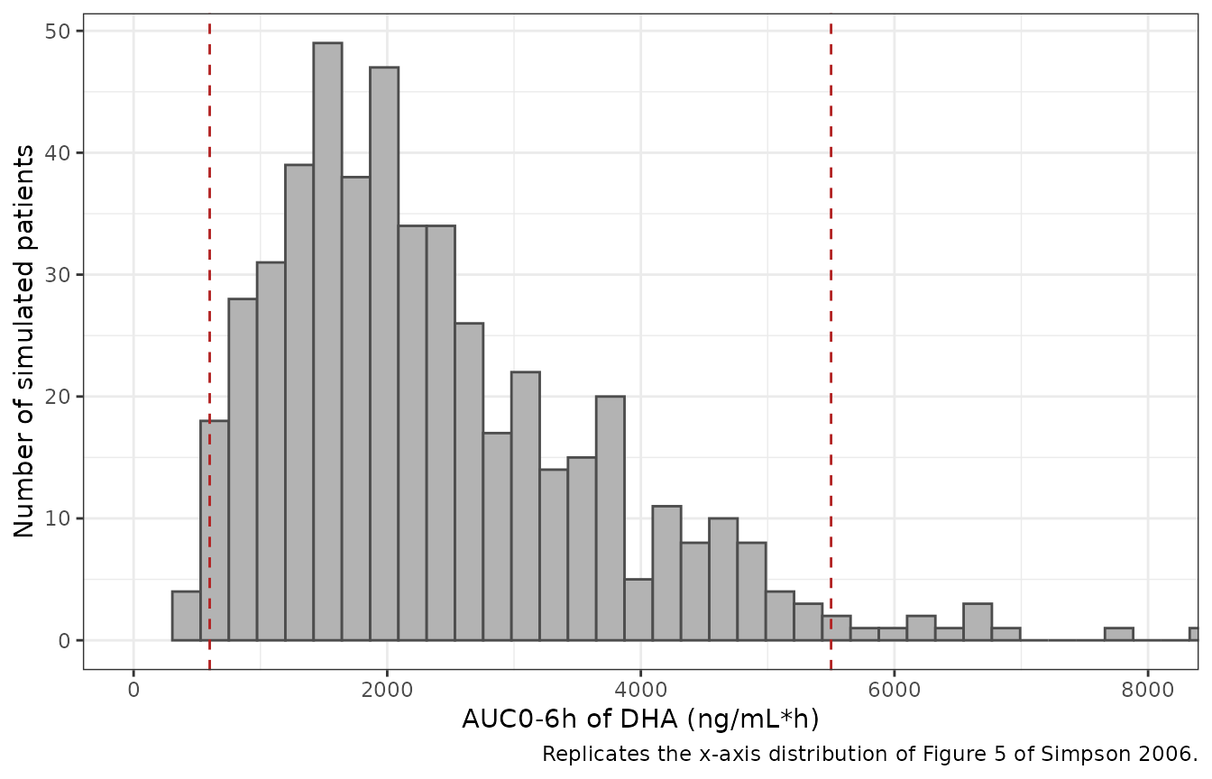
Simulated distribution of DHA AUC0-6h. Dashed lines mark the approximate span of the AUC0-6h values plotted on the x axis of Figure 5 of Simpson 2006.
auc06_q <- stats::quantile(nca$auc06_nghml, c(0.10, 0.50, 0.90))
auc06_q
#>      10%      50%      90%
#> 1052.672 2096.079 4056.708

# Realised 1,005 / 2,071 / 4,764 ng*h/mL at 16 threads. Figure 5's plotted
# points run from about 600 to 5,500 ng*h/mL. The bounds below admit cohort
# noise but still fail on a two-fold error in CL/F or dose, which would move
# the median to roughly 1,040 or 4,140.
stopifnot(
  auc06_q[["50%"]] > 1200, auc06_q[["50%"]] < 3500,
  auc06_q[["10%"]] > 500,
  auc06_q[["90%"]] < 8000
)
Comparison against published NCA
Simpson 2006 publishes no NCA or exposure summary
table for DHA. The only observed exposure statistic in the paper is the
“median (range) of the observed individual peak concentrations … 269
ng/ml (11-4,720 ng/ml)”, and that is for artesunate,
which the paper could not model and which this file therefore does not
contain. nlmixr2lib::ncaComparisonTable() is consequently
not used here: there is no published per-group Cmax / Tmax / AUC to
place beside the simulated column, and the only exposure quantity the
paper does report for DHA (AUC0-6h, Figure 5) is published as a scatter
of points rather than as summary statistics. That comparison is made
against the figure’s span above.
Every quantitative DHA statement the paper does make is collected in the gate below.
claims <- tibble::tribble(
  ~Claim, ~Source, ~Published, ~Model, ~Pass,
  "CL/F for a male (L/kg/h)", "Table 5",
  "3.17", sprintf("%.2f", typ$clkg[typ$SEXF == 0][1]),
  isTRUE(all.equal(typ$clkg[typ$SEXF == 0][1], 3.17, tolerance = 1e-6)),

  "CL/F for a female (L/kg/h)", "Table 5",
  "2.03", sprintf("%.2f", typ$clkg[typ$SEXF == 1][1]),
  isTRUE(all.equal(typ$clkg[typ$SEXF == 1][1], 2.03, tolerance = 1e-6)),

  "V/F at 15 kg (L/kg)", "Table 5",
  "1.81", sprintf("%.2f", typ$vckg[typ$WT == 15][1]),
  abs(typ$vckg[typ$WT == 15][1] - 1.81) < 0.005,

  "V/F at 70 kg (L/kg)", "Table 5",
  "6.34", sprintf("%.2f", typ$vckg[typ$WT == 70][1]),
  abs(typ$vckg[typ$WT == 70][1] - 6.34) < 0.005,

  "Base-model elimination half-life (min)", "Abstract / Results",
  "43", sprintf("%.1f", thalf_base_min),
  abs(thalf_base_min - 43) < 1,

  "Terminal slope equals the fixed appearance rate (1/h)", "Discussion",
  "0.20", sprintf("%.3f", -slope),
  abs(slope + 0.2) < 0.005,

  "AUC0-6h median inside the Figure 5 point cloud (ng*h/mL)", "Figure 5",
  "1,000-4,000", sprintf("%.0f", auc06_q[["50%"]]),
  auc06_q[["50%"]] > 1200 && auc06_q[["50%"]] < 3500,

  "AUC0-inf equals Dose / (CL/F)", "Model identity",
  "0% difference", sprintf("%.2f%% median", stats::median(auc_pct)),
  stats::median(auc_pct) < 0.5
)

claims |>
knitr::kable(caption = "Published claims against the packaged model.")| Claim | Source | Published | Model | Pass |
|---|---|---|---|---|
| CL/F for a male (L/kg/h) | Table 5 | 3.17 | 3.17 | TRUE |
| CL/F for a female (L/kg/h) | Table 5 | 2.03 | 2.03 | TRUE |
| V/F at 15 kg (L/kg) | Table 5 | 1.81 | 1.81 | TRUE |
| V/F at 70 kg (L/kg) | Table 5 | 6.34 | 6.34 | TRUE |
| Base-model elimination half-life (min) | Abstract / Results | 43 | 43.3 | TRUE |
| Terminal slope equals the fixed appearance rate (1/h) | Discussion | 0.20 | 0.200 | TRUE |
| AUC0-6h median inside the Figure 5 point cloud (ng*h/mL) | Figure 5 | 1,000-4,000 | 2096 | TRUE |
| AUC0-inf equals Dose / (CL/F) | Model identity | 0% difference | 0.02% median | TRUE |
Assumptions and deviations
- Only the DHA model is packaged. Simpson 2006 states plainly that the artesunate concentration-time data could not support a compartmental fit (“precluding formal pharmacokinetic modelling”, Results). There is no parent model to extract, so this file is a metabolite-only model whose dose is the administered artesunate amount.
- No molar correction between artesunate and DHA. The paper assumed complete conversion and “the exact dose (mg/kg) administered was used in the modelling” (Methods), so CL/F and V/F are expressed in artesunate-dose terms. The model file follows that convention exactly; do not apply the 284.35 / 384.42 molecular-weight ratio when dosing it.
-
Table 5 is a rendered image. The PMC record for
this article carries no machine-readable table markup, so every value in
ini()was read from the published table imagepmed.0030444.t005.jpgin the article’s PMC supplementary-files bundle. The four printed typical volumes give an independent arithmetic check on that reading, and Check 1 above runs it. -
The weight effect is affine, not allometric. The
Methods sentence about allometric scaling describes the covariate
screen; the final model of Table 5 is an intercept plus a linear
(WT/70)slope on the per-kilogram V/F, with no weight effect on CL/F. This is documented at length in the model file’sWTcovariate notes. -
Sex is stored as the canonical
SEXF(1 = female). The paper’s estimated coefficient is the increase in CL/F for a male, so the model applies it to(1 - SEXF). Table 5 prints both endpoints (3.17 male, 2.03 female) and 2.03 + 1.14 = 3.17, so neither the sign nor the reference category is ambiguous. -
Inter-individual and residual variability are read as
log-scale standard deviations, not as
log(CV^2 + 1)variances. The Methods define the reported %CV as “approximated by the square root of the variance estimate”, so the 62% / 75% / 93% figures are the log-scale SDs directly and the nlmixr2 variances are their squares. Using thelog(CV^2 + 1)conversion here would contradict the paper’s own definition. - The two etas are uncorrelated because “the data did not support a full variance-covariance matrix for the random effects of CL/F and V/F” (Results). The paper reports no covariance to encode.
-
ncaComparisonTable()is not used. As explained above, the paper publishes no DHA NCA table, and the one DHA exposure quantity it reports (AUC0-6h) is published only as a scatter plot. A comparison table built fromDose / CLwould be circular. The published-claims table is used instead. - Cohort construction. Body weights are drawn from per-site normal distributions truncated to the published per-site ranges (Table 2 gives mean, SD and range but not the distributional shape), sex from the published per-site percent-male, and dose from the published per-site mean mg/kg. Age is not a covariate in the final model and is not simulated. Sampling times are a dense regular grid rather than the trials’ actual (partly randomised, partly sparse) schedules, because the purpose here is to characterise the model rather than to reproduce the estimation data set.
-
No parameter was tuned. Every
ini()value is the published Table 5 value; the base-model re-ini()in Check 2 uses only the published base-model CL/F and V/F and is used for validation, not shipped.