Rezafungin (Rubino 2021)
Source:vignettes/articles/Rubino_2021_rezafungin.Rmd
Rubino_2021_rezafungin.RmdModel and source
- Citation: Rubino CM, Flanagan S. Population pharmacokinetics of rezafungin in patients with fungal infections. Antimicrob Agents Chemother. 2021;65(11):e00842-21. doi:10.1128/AAC.00842-21
- Description: Four-compartment population PK model for rezafungin after IV infusion in healthy subjects (three phase 1 studies) and in patients with candidemia and/or invasive candidiasis (phase 2 STRIVE) (Rubino 2021), with serum-albumin power effects on CL and the first peripheral volume, a female-sex shift on CL, a linear body-surface-area slope on the central volume, BSA power effects on both first and second peripheral volumes, and infection-status shifts on the central and second peripheral volumes.
- Article: Antimicrob Agents Chemother 2021;65(11):e00842-21 (open access)
A later analysis of the same drug that adds the phase 3 ReSTORE trial
and hepatically impaired subjects is available as
readModelDb("Roepcke_2023_rezafungin"); it uses a
three-compartment structure and a different covariate set, and is a
separate model rather than an update of this one.
Population
Rezafungin is a once-weekly intravenous echinocandin. Rubino 2021 pooled 1,518 plasma concentrations from 135 subjects: 66 healthy subjects from three phase 1 studies (a single-ascending-dose study of 50-400 mg, a multiple-ascending-dose study of 100-400 mg weekly, and a QTcF study of 600 and 1,400 mg) and 69 patients with candidemia and/or invasive candidiasis from the phase 2 STRIVE trial (NCT02734862), who received 400 mg once weekly or 400 mg in week 1 followed by 200 mg weekly. Phase 1 infusions ran 60 min (SAD, MAD) or at 400 mg/h (QTcF).
The phase 1 subjects were younger (median age 36-44.5 years) than the STRIVE patients (median 57.5 years, range 24-88), and had much higher serum albumin (median 4.76-4.87 g/dL versus 2.81 g/dL, range 1.62-4.97). Body size was similar across studies (median BSA 1.81-1.83 m^2). Overall 44.9% of subjects were female and 86% White. STRIVE enrolled patients with severe renal impairment, with creatinine clearance down to 8.57 mL/min/1.73 m^2. Source: Rubino 2021 Table 1.
The structural model is the four-compartment model (a central and three peripheral compartments) with zero-order IV input and linear elimination developed earlier from phase 1 data (Lakota 2018), refitted without that model’s body-weight scaling. The covariate analysis retained serum albumin (on CL and Vp1), sex (on CL), BSA (on Vc, Vp1 and Vp2) and infection status (on Vc and Vp2). IIV is on CL, Vc and Vp1, with CL correlated with both Vc and Vp1; IIV on Vp2 reuses the Vp1 random effect multiplied by an estimated scaling term. The residual error is proportional.
The same information is available programmatically via
rxode2::rxode(readModelDb("Rubino_2021_rezafungin"))$population.
Source trace
Every numeric value in ini() carries an in-file comment
pointing to its source. The table collects them in one place. All values
are from Rubino 2021 Table 2 and the equations in its footnote a.
| Equation / parameter | Value | Source location |
|---|---|---|
lcl (CL) |
0.254 L/h | Table 2, ‘CL, liter/h’ (3.74 %SEM) |
e_alb_cl |
-0.844 | Table 2, ‘CL-albumin power’ (9.34 %SEM) |
e_sexf_cl |
-0.133 | Table 2, ‘Proportional change in females’ (24.3 %SEM) |
lvc (Vc) |
11.1 L | Table 2, ‘Vc, liter’ (8.87 %SEM) |
e_bsa_vc |
7.54 L per m^2 | Table 2, ‘Vc-BSA slope’ (23.6 %SEM) |
e_infect_vc |
0.478 | Table 2, ‘Proportional change in infected patients’ under Vc (27.7 %SEM) |
lq (CLd1) |
18.2 L/h | Table 2, ‘CLd1, liter/h’ (1.09 %SEM) |
lvp (Vp1) |
14.6 L | Table 2, ‘Vp1, liter’ (4.42 %SEM) |
e_alb_vp |
-0.829 | Table 2, ‘Vp1-albumin power’ (10.6 %SEM) |
e_bsa_vp |
1.14 | Table 2, ‘Vp1-BSA power’ (15.6 %SEM) |
lq2 (CLd2) |
0.541 L/h | Table 2, ‘CLd2, liter/h’ (8.11 %SEM) |
lvp2 (Vp2) |
6.69 L | Table 2, ‘Vp2, liter’ (11.8 %SEM) |
e_bsa_vp2 |
2.47 | Table 2, ‘Vp2-BSA power’ (18.4 %SEM) |
e_infect_vp2 |
1.69 | Table 2, ‘Proportional change in infected patients’ under Vp2 (19.5 %SEM) |
vp2_eta_scale |
1.71 | Table 2, ‘IIV scaling term relative to Vp1 IIV’ (18.8 %SEM) |
lq3 (CLd3) |
0.0743 L/h | Table 2, ‘CLd3, liter/h’ (7.62 %SEM) |
lvp3 (Vp3) |
13.6 L | Table 2, ‘Vp3, liter’ (8.38 %SEM) |
etalcl variance |
0.0562 | Table 2, IIV on CL, 0.0562 (23.7%) |
etalvc variance |
0.148 | Table 2, IIV on Vc, 0.148 (38.5%) |
etalvp variance |
0.0471 | Table 2, IIV on Vp1, printed %CV 21.7%; see Assumptions |
etalcl-etalvc covariance |
0.0604 | Table 2, ‘Covariance between CL and Vc’ (14.1 %SEM) |
etalcl-etalvp covariance |
0.0107 | Table 2, ‘Covariance between CL and Vp1’ (51.8 %SEM) |
propSd |
0.0891 | Table 2, ‘Proportional error, %CV’ = 8.91 (2.57 %SEM) |
| CL equation | 0.254 (1 - 0.133 SEXF) (alb/4.2)^-0.844 |
Table 2 footnote a |
| Vc equation | [11.1 + 7.54 (BSA - 1.83)] (1 + 0.478 infected) |
Table 2 footnote a |
| Vp1 equation | 14.6 (alb/4.2)^-0.829 (BSA/1.83)^1.14 |
Table 2 footnote a |
| Vp2 equation | 6.69 (1 + 1.69 infected) (BSA/1.83)^2.47 |
Table 2 footnote a |
| Four-compartment IV structure | – | Results, ‘Population pharmacokinetic model development’; Methods |
The IIV block is checked for positive definiteness before any simulation:
ui <- rxode2::rxode(readModelDb("Rubino_2021_rezafungin"))
#> ℹ parameter labels from comments will be replaced by 'label()'
omega <- ui$omega
stopifnot(all(eigen(omega, only.values = TRUE)$values > 0))
# %CV convention of Table 2 is sqrt(omega^2): 23.7%, 38.5%, 21.7%.
round(100 * sqrt(diag(omega)), 1)
#> etalvp etalcl etalvc
#>   21.7   23.7   38.5
Virtual cohort
The validation targets are the STRIVE patients (Table 3) and the
subgroup comparisons of Figure 1, so the main cohort is STRIVE-like:
every patient infected (DIS_INFECT_ACTIVE = 1), 40% female,
and BSA and albumin drawn from normal distributions with the STRIVE mean
and SD of Table 1, truncated to the published range. Two arms of 200
patients follow the two STRIVE regimens for three weekly doses; both
receive 400 mg in week 1, which is the interval Table 3 summarises.
Doses are 1-h IV infusions (the STRIVE infusion duration is not given in
Rubino 2021; 1 h matches the phase 1 400 mg regimens).
set.seed(20210816)
rxode2::rxSetSeed(20210816)

n_per_arm <- 200L

rtnorm <- function(n, mean, sd, lo, hi) {
  pmin(pmax(stats::rnorm(n, mean, sd), lo), hi)
}

make_arm <- function(n, doses, arm, id_offset) {
  subj <- tibble::tibble(
    id = id_offset + seq_len(n),
    arm = arm,
    BSA = rtnorm(n, 1.83, 0.257, 1.22, 2.37),
    # Albumin in g/dL from Table 1, converted to the canonical g/L.
    ALB = 10 * rtnorm(n, 2.82, 0.647, 1.62, 4.97),
    SEXF = stats::rbinom(n, 1, 0.40),
    DIS_INFECT_ACTIVE = 1L
  )
  dose_rows <- tidyr::crossing(subj, tibble::tibble(time = c(0, 168, 336), amt = doses)) |>
    mutate(evid = 1L, cmt = "central", dur = 1)
  obs_times <- sort(unique(c(
    seq(0, 2, by = 0.25), seq(3, 24, by = 1), seq(26, 504, by = 4), 168, 336
  )))
  obs_rows <- tidyr::crossing(subj, time = obs_times) |>
    mutate(amt = NA_real_, evid = 0L, cmt = "central", dur = NA_real_)
  bind_rows(dose_rows, obs_rows) |>
    arrange(id, time, desc(evid))
}

events <- bind_rows(
  make_arm(n_per_arm, c(400, 400, 400), "400 mg weekly", 0L),
  make_arm(n_per_arm, c(400, 200, 200), "400 mg then 200 mg weekly", n_per_arm)
)
stopifnot(!anyDuplicated(unique(events[, c("id", "time", "evid")])))
stopifnot(dplyr::n_distinct(events$id) == 2L * n_per_arm)
Simulation
mod <- readModelDb("Rubino_2021_rezafungin")
sim <- rxode2::rxSolve(
  mod, events,
  keep = c("arm", "BSA", "ALB", "SEXF"),
  returnType = "data.frame"
)
#> ℹ parameter labels from comments will be replaced by 'label()'
stopifnot(dplyr::n_distinct(sim$id) == 2L * n_per_arm)

# The stochastic solve must carry IIV: individual CL should vary with
# roughly the published 23.7% CV plus the covariate spread.
cl_i <- sim |> distinct(id, cl) |> pull(cl)
stopifnot(stats::sd(log(cl_i)) > 0.15)
Replicate published figures
Concentration-time profiles in STRIVE patients
Rubino 2021 Figure 3 is a prediction-corrected VPC against the observed STRIVE data, which are not published. The plot below shows the simulated median and 5th-95th percentiles for the two STRIVE regimens over three weeks.
sim |>
  filter(time > 0) |>
  group_by(arm, time) |>
  summarise(
    p05 = quantile(Cc, 0.05), p50 = median(Cc), p95 = quantile(Cc, 0.95),
    .groups = "drop"
  ) |>
  ggplot(aes(time / 24, p50, colour = arm, fill = arm)) +
  geom_ribbon(aes(ymin = p05, ymax = p95), alpha = 0.2, colour = NA) +
  geom_line() +
  scale_y_log10() +
  labs(
    x = "Time since first dose (day)", y = "Rezafungin plasma concentration (mg/L)",
    colour = NULL, fill = NULL,
    caption = "Simulated median and 90% prediction interval; cf. Figure 3 of Rubino 2021."
  ) +
  theme_bw() +
  theme(legend.position = "bottom")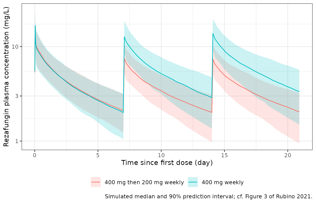
Figure 1 – covariate effects on week-1 AUC
Figure 1 of Rubino 2021 shows simulated week-1 AUC(0-168h) for seven subject types relative to an infected male with BSA 1.83 m^2 and albumin 2.8 g/dL. The chunk below computes the same ratios for typical subjects (no IIV) after a single 400 mg 1-h infusion. The published values are the box medians, read by eye from the figure to about +/-5 percentage points.
scenarios <- tibble::tribble(
  ~label,                             ~DIS_INFECT_ACTIVE, ~SEXF, ~ALB_gdL, ~BSA, ~published_pct,
  "Reference: infected male",          1L,                0L,    2.8,      1.83,  0,
  "Uninfected, male, alb 4.77 g/dL",   0L,                0L,    4.77,     1.83,  60,
  "Uninfected, female, alb 4.77 g/dL", 0L,                1L,    4.77,     1.83,  70,
  "Infected, male, alb 3.9 g/dL",      1L,                0L,    3.9,      1.83,  19,
  "Infected, male, alb 1.9 g/dL",      1L,                0L,    1.9,      1.83,  -19,
  "Infected, female, BSA 2.37 m^2",    1L,                1L,    2.8,      2.37,  -14,
  "Infected, female, BSA 1.22 m^2",    1L,                1L,    2.8,      1.22,  41,
  "Infected, female, alb 2.8 g/dL",    1L,                1L,    2.8,      1.83,  7
) |>
  mutate(id = row_number(), ALB = 10 * ALB_gdL)

tv_times <- sort(unique(c(seq(0, 2, by = 0.05), seq(2, 168, by = 0.5))))
tv_events <- bind_rows(
  scenarios |> mutate(time = 0, amt = 400, evid = 1L, cmt = "central", dur = 1),
  tidyr::crossing(scenarios, time = tv_times) |>
    mutate(amt = NA_real_, evid = 0L, cmt = "central", dur = NA_real_)
) |>
  arrange(id, time, desc(evid))

tv_sim <- rxode2::rxSolve(
  rxode2::zeroRe(mod), tv_events,
  keep = "label", returnType = "data.frame"
)
#> ℹ parameter labels from comments will be replaced by 'label()'
#> ℹ omega/sigma items treated as zero: 'etalvp', 'etalcl', 'etalvc'
#> Warning: multi-subject simulation without without 'omega'
stopifnot(dplyr::n_distinct(tv_sim$id) == nrow(scenarios))

trap <- function(t, y) sum(diff(t) * (head(y, -1) + tail(y, -1)) / 2)
tv_auc <- tv_sim |>
  group_by(id, label) |>
  summarise(auc168 = trap(time, Cc), .groups = "drop") |>
  left_join(select(scenarios, id, published_pct), by = "id") |>
  mutate(simulated_pct = 100 * (auc168 / auc168[id == 1] - 1))

tv_auc |>
  mutate(auc168 = signif(auc168, 4), simulated_pct = round(simulated_pct, 1)) |>
  select(label, auc168, simulated_pct, published_pct) |>
  dplyr::rename(
    "Subject type" = label,
    "Typical AUC0-168 (mg*h/L)" = auc168,
    "Simulated change (%)" = simulated_pct,
    "Figure 1 median (%)" = published_pct
  ) |>
knitr::kable(caption = "Replicates Figure 1 of Rubino 2021 with typical-value solves.")| Subject type | Typical AUC0-168 (mg*h/L) | Simulated change (%) | Figure 1 median (%) |
|---|---|---|---|
| Reference: infected male | 697.3 | 0.0 | 0 |
| Uninfected, male, alb 4.77 g/dL | 1113.0 | 59.6 | 60 |
| Uninfected, female, alb 4.77 g/dL | 1185.0 | 70.0 | 70 |
| Infected, male, alb 3.9 g/dL | 824.5 | 18.2 | 19 |
| Infected, male, alb 1.9 g/dL | 559.1 | -19.8 | -19 |
| Infected, female, BSA 2.37 m^2 | 597.8 | -14.3 | -14 |
| Infected, female, BSA 1.22 m^2 | 966.6 | 38.6 | 41 |
| Infected, female, alb 2.8 g/dL | 742.4 | 6.5 | 7 |
# Deterministic check: every subgroup lands within the figure-reading
# tolerance of the published box median. A sign error on any covariate
# exponent, or the infection effect placed on the wrong volume, moves one or
# more rows by 20 or more percentage points.
stopifnot(all(abs(tv_auc$simulated_pct - tv_auc$published_pct) < 5))
PKNCA validation
Table 3 of Rubino 2021 summarises, for the 68 STRIVE patients,
AUC(0-168h), Cmax and Cmin over the first dosing interval, computed from
profiles simulated with each patient’s post hoc parameters. Cmin is the
lowest concentration of that interval, which for a declining profile is
the concentration at 168 h; it is computed here as
clast.obs over [0, 168 h] (PKNCA’s cmin over
that interval would return the pre-dose zero).
sim_nca <- sim |>
  filter(!is.na(Cc)) |>
  select(id, arm, time, Cc)

# Guarantee one time = 0 record per subject (pre-infusion concentration 0).
sim_nca <- bind_rows(
  sim_nca,
  sim_nca |> distinct(id, arm) |> mutate(time = 0, Cc = 0)
) |>
  distinct(id, arm, time, .keep_all = TRUE) |>
  arrange(id, arm, time)

conc_obj <- PKNCA::PKNCAconc(sim_nca, Cc ~ time | arm + id)
dose_df <- events |>
  filter(evid == 1, time == 0) |>
  select(id, arm, time, amt)
dose_obj <- PKNCA::PKNCAdose(dose_df, amt ~ time | arm + id)

intervals <- data.frame(
  start = 0, end = 168,
  cmax = TRUE, tmax = TRUE, auclast = TRUE, clast.obs = TRUE
)
nca_res <- PKNCA::pk.nca(PKNCA::PKNCAdata(conc_obj, dose_obj, intervals = intervals))
Comparison against published NCA
Table 3 reports mean (SD) and median (range) over the pooled STRIVE
patients, and both arms receive the same 400 mg dose in week 1, so the
published median is the reference for each arm.
ncaComparisonTable() summarises the simulated per-subject
values by their median.
published <- tibble::tribble(
  ~arm,                         ~cmax, ~auclast, ~clast.obs,
  "400 mg weekly",              16.4,  673,      1.90,
  "400 mg then 200 mg weekly",  16.4,  673,      1.90
)

cmp <- nlmixr2lib::ncaComparisonTable(
  simulated = nca_res,
  reference = published,
  by = "arm",
  units = c(cmax = "mg/L", auclast = "mg*h/L", clast.obs = "mg/L"),
  tolerance_pct = 20
)
knitr::kable(
  cmp,
  caption = paste(
    "Simulated vs. Rubino 2021 Table 3 (medians, n = 68 STRIVE patients) for",
    "the first dosing interval after 400 mg. auclast = AUC(0-168h);",
    "clast.obs = Cmin (concentration at 168 h). * differs by >20%."
  )
)| NCA parameter | arm | Reference | Simulated | % diff |
|---|---|---|---|---|
| Cmax (mg/L) | 400 mg weekly | 16.4 | 16.7 | +2.0% |
| Cmax (mg/L) | 400 mg then 200 mg weekly | 16.4 | 16.4 | +0.2% |
| Clast (mg/L) | 400 mg weekly | 1.9 | 2 | +5.3% |
| Clast (mg/L) | 400 mg then 200 mg weekly | 1.9 | 2.1 | +10.6% |
| AUClast (mg*h/L) | 400 mg weekly | 673 | 700 | +4.0% |
| AUClast (mg*h/L) | 400 mg then 200 mg weekly | 673 | 705 | +4.8% |
nca_df <- as.data.frame(nca_res) |>
  filter(PPTESTCD %in% c("cmax", "auclast", "clast.obs")) |>
  select(id, arm, PPTESTCD, PPORRES)

ref_vals <- c(cmax = 16.4, auclast = 673, clast.obs = 1.90)
pct_diff <- nca_df |>
  group_by(PPTESTCD) |>
  summarise(median = median(PPORRES), .groups = "drop") |>
  mutate(pct = 100 * (median / ref_vals[PPTESTCD] - 1))
pct_diff
#> # A tibble: 3 × 3
#>   PPTESTCD  median   pct
#>   <chr>      <dbl> <dbl>
#> 1 auclast   702.   4.35
#> 2 clast.obs   2.07 8.95
#> 3 cmax       16.5  0.687

# Structural check on the cohort centre (robust to which subjects land in
# the tails; see the package's vignette-assertion guidance).
stopifnot(
  nrow(pct_diff) == 3L,
  all(abs(pct_diff$pct) < 15)
)
Model-based CL and Vss are read directly off the simulated individual parameters, as Rubino 2021 derives them from the post hoc estimates.
params <- sim |>
  distinct(id, arm, cl, vc, vp, vp2, vp3) |>
  mutate(Vss = vc + vp + vp2 + vp3, V123 = vc + vp + vp2)

params |>
  summarise(
    across(c(cl, Vss, V123), list(median = median, mean = mean))
  ) |>
  tidyr::pivot_longer(everything(), names_to = c("parameter", "stat"), names_sep = "_") |>
  tidyr::pivot_wider(names_from = stat, values_from = value) |>
  left_join(
    tibble::tribble(
      ~parameter, ~pub_median, ~pub_mean,
      "cl",       0.345,       0.365,
      "Vss",      52.7,        61.0,
      "V123",     52.7,        61.0
    ),
    by = "parameter"
  ) |>
  mutate(across(where(is.numeric), ~ signif(.x, 3))) |>
  dplyr::rename(
    "Parameter" = parameter,
    "Simulated median" = median, "Simulated mean" = mean,
    "Table 3 median" = pub_median, "Table 3 mean" = pub_mean
  ) |>
knitr::kable(caption = "Model-based CL (L/h) and volume (L) vs. Rubino 2021 Table 3.")| Parameter | Simulated median | Simulated mean | Table 3 median | Table 3 mean |
|---|---|---|---|---|
| cl | 0.337 | 0.362 | 0.345 | 0.365 |
| Vss | 68.600 | 72.000 | 52.700 | 61.000 |
| V123 | 55.000 | 58.400 | 52.700 | 61.000 |
Clearance and every exposure metric reproduce Table 3. Table 3’s Vss (median 52.7 L) does not: the sum of all four model volumes is about 25-30% higher, whereas the sum of Vc, Vp1 and Vp2 matches it closely. The source does not define how Vss was computed, and the exposure metrics, which depend on all four compartments, agree with the published values, so this looks like a Vss definition that leaves out the deep compartment Vp3 (13.6 L) rather than a problem with the parameters.
Assumptions and deviations
- IIV variance on Vp1. Table 2 prints the Vp1 variance as 0.0107, the same number as the CL-Vp1 covariance on the row above it. That value is inconsistent with the paper’s own %CV for it (21.7%; the paper’s %CV is sqrt(omega^2), as the CL and Vc rows show: sqrt(0.0562) = 23.7%, sqrt(0.148) = 38.5%) and with the printed CL-Vp1 r^2 of 0.043 (which gives 0.0107^2 / (0.0562 x 0.043) = 0.0474). The model uses 0.217^2 = 0.0471.
- CL-Vc r^2. Table 2 prints r^2 = 0.4638 for the CL-Vc covariance; the printed variances and covariance give 0.0604^2 / (0.0562 x 0.148) = 0.4386, so 0.4638 is probably a transposition of digits. The covariance 0.0604 is used as printed. Vc and Vp1 have no covariance in the final model.
- Vp2 IIV. Table 2 reports no separate IIV for Vp2 and states that it was “estimated relative to the IIV in Vp1”; the model applies the Vp1 eta multiplied by the estimated scaling term 1.71 (a perfectly correlated random effect with SD 1.71 x 0.217 = 0.37).
- Infection effect on Vp2, not Vp1. The Discussion describes infection status as a predictor of Vc and Vp1, but Table 2 lists the second ‘proportional change in infected patients’ under Vp2 and the footnote-a equation places it on Vp2. The equation is followed. Placing it on Vp1 would drop the typical STRIVE AUC(0-168h) to about 570 mg*h/L against the published 673, and would miss the Figure 1 ratios.
-
Albumin units and normalization. Albumin enters in
g/dL with a 4.2 g/dL reference; the canonical
ALBcolumn is g/L and the model converts internally. The paper normalized albumin “for variable interlaboratory reference ranges” without giving the formula, so the model takes albumin as supplied. -
Infection status. The paper’s ‘infected’ indicator
(phase 2 STRIVE patients with candidemia and/or invasive candidiasis) is
encoded as
DIS_INFECT_ACTIVE = 1; healthy phase 1 subjects are 0. - BSA formula. Not stated in the source.
- STRIVE infusion duration. Not stated in Rubino 2021; 1 h is assumed.
- Virtual cohort. BSA and albumin were drawn independently from truncated normal distributions with the STRIVE mean and SD of Table 1; their correlation in the real cohort is not reported.
- Figure 1 values were read by eye from the published box medians, to about +/-5 percentage points.
- Table 1 STRIVE weight range. Printed as ‘34-55’ kg against a mean of 74.5 kg (SD 21.3), which is a typesetting error; it is not used.
- Errata. No correction notice for this article was found in a Europe PMC search (2026-09-29).