Bee venom phospholipase A2 (Chae 2025)
Source:vignettes/articles/Chae_2025_beeVenomPLA2.Rmd
Chae_2025_beeVenomPLA2.RmdModel and source
- Citation: Chae SU, Min JS, Jo SJ, Lee CB, Park J, Bae SH, Bae SK. Prediction of first-in-human dose for new composition bee venom based on allometric scaling and pharmacokinetic modeling approach. Transl Clin Pharmacol. 2025;33(1):27-39. doi:10.12793/tcp.2025.33.e4
- Article: https://doi.org/10.12793/tcp.2025.33.e4 (open access, PMC11976151)
Chae 2025 developed a new composition bee venom (NCBV), enriched in bee venom phospholipase A2 (bvPLA2), for Alzheimer’s disease and predicted its first-in-human (FIH) subcutaneous dose. Plasma bvPLA2 after a single subcutaneous (SC) NCBV injection was fitted separately in three species, each with a two-compartment model with first-order absorption (Figure 1, Table 2), and the three parameter sets were scaled to a 70 kg human by three allometric methods (Table 3). The paper therefore contributes six model files:
| Model | Species | Basis |
|---|---|---|
Chae_2025_beeVenomPLA2_mouse |
ICR mouse | population PK fit, Table 2 |
Chae_2025_beeVenomPLA2_rat |
Sprague-Dawley rat | population PK fit, Table 2 |
Chae_2025_beeVenomPLA2_dog |
beagle dog | population PK fit, Table 2 |
Chae_2025_beeVenomPLA2_human_simple |
human (projected) | simple allometry, Table 3 |
Chae_2025_beeVenomPLA2_human_brw |
human (projected) | brain-weight corrected allometry, Table 3 (the paper’s recommended method) |
Chae_2025_beeVenomPLA2_human_mlp |
human (projected) | maximum-lifespan-potential corrected allometry, Table 3 |
All parameters are apparent (divided by the unknown SC bioavailability F). The animal models are per kg body weight, so their doses are given in mg/kg; the human projections take doses in mg. Concentrations are in ng/mL.
Population
- Mice: male and female ICR mice (7-8 weeks, 20-35 g), a single 0.5 mg/kg SC dose, terminal cardiac-puncture sampling with 4 animals per time point (48 per sex) from 0.05 to 24 h.
- Rats: male and female Sprague-Dawley rats (7-9 weeks, 200-330 g), 0.2, 0.5, 1 and 2 mg/kg SC, 4 per sex per dose, serial sampling to 24 h. An IV arm gave SC bioavailability of 11.9-18.4% (Table 1); the model itself is apparent.
- Beagle dogs: 0.3, 0.6 and 0.9 mg/kg SC, 4 per sex per dose, sampling at 0.25-24 h.
- Humans: no human data; the three human files are forward projections for a 70 kg adult.
bvPLA2 was measured by ELISA (calibration range 0.78-100 ng/mL). The
same information is available programmatically, for example
readModelDb("Chae_2025_beeVenomPLA2_rat")()$population.
Source trace
| Equation / parameter | Mouse | Rat | Dog | Source location |
|---|---|---|---|---|
| Two-compartment model, first-order absorption and elimination | Methods “PK model development”; Figure 1 | |||
lka (ka, 1/h) |
9.08 | 0.803 | 0.544 | Table 2 |
lcl (CL/F, L/h/kg) |
0.243 | 1.83 | 0.150 | Table 2 |
lvc (Vc/F, L/kg) |
0.912 | 0.712 | 0.385 | Table 2 |
lvp (Vp/F, L/kg) |
5.89 | 6.89 | 1.47 | Table 2 |
lq (Q/F, L/h/kg) |
0.121 | 0.862 | 0.141 | Table 2 |
etalcl (variance; CV%) |
0.01806 (13.5%) | 0.4186 (72.1%) | 0.07393 (27.7%) | Table 2 BSV |
etalq |
- | 0.3479 (64.5%) | - | Table 2 BSV |
etalka |
- | 0.1181 (35.4%) | - | Table 2 BSV |
etalvc |
- | - | 0.1547 (40.9%) | Table 2 BSV |
propSd |
0.327 | 0.322 | 0.166 | Table 2 sigma prop |
| Parameter | Simple | BrW | MLP | Source location |
|---|---|---|---|---|
lcl (CL/F, L/h) |
12.9 | 3.25 | 0.612 | Table 3 |
lvc (Vc/F, L) |
19.5 | 4.92 | 10.0 | Table 3 |
lvp (Vp/F, L) |
67.3 | 17.0 | 34.7 | Table 3 |
lq (Q/F, L/h) |
14.7 | 3.72 | 7.59 | Table 3 |
lka (1/h) |
0.803 | 0.803 | 0.803 | rat Table 2 value; back-solved against Table 4 (below) |
e_wt_cl, e_wt_vc, e_wt_vp,
e_wt_q
|
0.847, 0.842, 0.729, 0.971 | - | - | Results, “Allometric scaling for the prediction of human PK parameters” |
propSd |
0 (fixed) | 0 (fixed) | 0 (fixed) | not reported for the projections |
BSV is reported as CV%; the log-normal variances are
log(CV^2 + 1).
Animal models: visual predictive checks
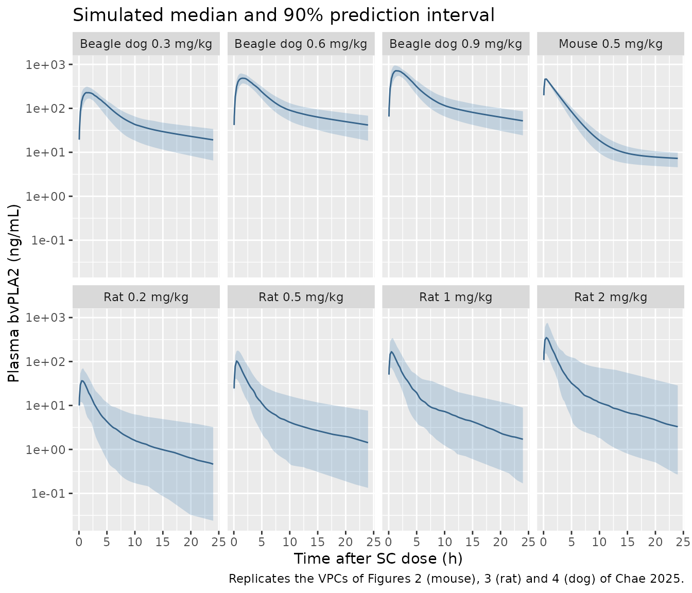
Each species is simulated at its studied doses, 100 virtual animals per dose group, to mirror the VPCs of Figures 2-4.
make_animal <- function(model, species, doses, n = 100L) {
  obs_times <- sort(unique(c(0, 0.05, 0.08, 0.25, 0.5, 1, 1.5, 2, 3, 4, 6, 8, 10, 24, seq(0, 24, by = 0.25))))
  ev <- lapply(seq_along(doses), function(i) {
    ids <- (i - 1L) * n + seq_len(n)
    dose_rows <- data.frame(id = ids, time = 0, evid = 1L, amt = doses[i], cmt = "depot")
    obs_rows <- expand.grid(id = ids, time = obs_times)
    obs_rows$evid <- 0L
    obs_rows$amt <- 0
    obs_rows$cmt <- "central"
    out <- rbind(dose_rows, obs_rows[, names(dose_rows)])
    out$dose_group <- paste(doses[i], "mg/kg")
    out
  })
  ev <- dplyr::bind_rows(ev) |> dplyr::arrange(id, time, dplyr::desc(evid))
  rxode2::rxSetSeed(2025)
  sim <- rxode2::rxSolve(readModelDb(model), events = ev, keep = "dose_group")
  sim <- as.data.frame(sim)
  sim$species <- species
  sim$dose_group <- factor(sim$dose_group, levels = paste(doses, "mg/kg"))
  list(events = ev, sim = sim)
}

mouse <- make_animal("Chae_2025_beeVenomPLA2_mouse", "Mouse", 0.5)
#> ℹ parameter labels from comments will be replaced by 'label()'
rat <- make_animal("Chae_2025_beeVenomPLA2_rat", "Rat", c(0.2, 0.5, 1, 2))
#> ℹ parameter labels from comments will be replaced by 'label()'
dog <- make_animal("Chae_2025_beeVenomPLA2_dog", "Beagle dog", c(0.3, 0.6, 0.9))
#> ℹ parameter labels from comments will be replaced by 'label()'
vpc_summary <- function(sim) {
  sim |>
    dplyr::group_by(species, dose_group, time) |>
    dplyr::summarise(
      Q05 = quantile(Cc, 0.05, na.rm = TRUE),
      Q50 = quantile(Cc, 0.50, na.rm = TRUE),
      Q95 = quantile(Cc, 0.95, na.rm = TRUE),
      .groups = "drop"
    )
}
vpc <- dplyr::bind_rows(vpc_summary(mouse$sim), vpc_summary(rat$sim), vpc_summary(dog$sim)) |>
  dplyr::filter(time > 0) |>
  dplyr::mutate(panel = paste(species, dose_group))

ggplot(vpc, aes(time, Q50)) +
  geom_ribbon(aes(ymin = Q05, ymax = Q95), alpha = 0.25, fill = "steelblue") +
  geom_line(colour = "steelblue4") +
  facet_wrap(~panel, ncol = 4) +
  scale_y_log10() +
  labs(
    x = "Time after SC dose (h)", y = "Plasma bvPLA2 (ng/mL)",
    title = "Simulated median and 90% prediction interval",
    caption = "Replicates the VPCs of Figures 2 (mouse), 3 (rat) and 4 (dog) of Chae 2025."
  )
PKNCA against the observed NCA (Table 1)
Table 1 reports non-compartmental parameters of the observed data (AUC to the last sample at 24 h, terminal half-life, Cmax, Tmax). The simulation is sampled at the study schedule (mice and rats 0.05-24 h, dogs 0.25-24 h) and analysed with PKNCA.
study_times <- list(
  Mouse = c(0, 0.05, 0.08, 0.25, 0.5, 1, 1.5, 2, 3, 4, 6, 8, 10, 24),
  Rat = c(0, 0.05, 0.08, 0.25, 0.5, 1, 1.5, 2, 3, 4, 6, 8, 10, 24),
  "Beagle dog" = c(0, 0.25, 0.5, 1, 2, 4, 8, 24)
)
animal_sim <- dplyr::bind_rows(mouse$sim, rat$sim, dog$sim) |>
  dplyr::mutate(treatment = paste(species, dose_group), dose_group = as.character(dose_group))
animal_nca_conc <- animal_sim |>
  dplyr::filter(!is.na(Cc)) |>
  dplyr::filter(
    (species == "Beagle dog" & time %in% study_times[["Beagle dog"]]) |
      (species != "Beagle dog" & time %in% study_times[["Mouse"]])
  ) |>
  dplyr::select(id, time, Cc, treatment)
animal_dose <- animal_sim |>
  dplyr::distinct(id, treatment, dose_group) |>
  dplyr::mutate(time = 0, amt = as.numeric(sub(" mg/kg", "", dose_group)))

conc_obj <- PKNCA::PKNCAconc(animal_nca_conc, Cc ~ time | treatment + id)
dose_obj <- PKNCA::PKNCAdose(animal_dose, amt ~ time | treatment + id)
intervals <- data.frame(start = 0, end = 24, cmax = TRUE, tmax = TRUE, auclast = TRUE, half.life = TRUE)
animal_nca <- PKNCA::pk.nca(PKNCA::PKNCAdata(conc_obj, dose_obj, intervals = intervals))

# Table 1 of Chae 2025; AUC converted from ug*h/mL to ng*h/mL.
published_t1 <- tibble::tribble(
  ~treatment, ~cmax, ~tmax, ~auclast, ~half.life,
  "Mouse 0.5 mg/kg", 474, 0.5, 1280, 2.24,
  "Rat 0.2 mg/kg", 68.2, 0.5, 101, 1.05,
  "Rat 0.5 mg/kg", 113, 0.25, 209, 1.89,
  "Rat 1 mg/kg", 231, 0.25, 586, 3.13,
  "Rat 2 mg/kg", 439, 0.5, 1220, 4.17,
  "Beagle dog 0.3 mg/kg", 354, 1, 1350, 3.29,
  "Beagle dog 0.6 mg/kg", 477.4, 1, 2290, 3.11,
  "Beagle dog 0.9 mg/kg", 680, 2, 3150, 2.93
)
cmp_t1 <- nlmixr2lib::ncaComparisonTable(
  simulated = animal_nca,
  reference = published_t1,
  by = "treatment",
  units = c(cmax = "ng/mL", tmax = "h", auclast = "ng*h/mL", half.life = "h"),
  tolerance_pct = 20
)
knitr::kable(cmp_t1, caption = "Simulated (median of 100 animals per group) vs. Table 1 observed NCA. * differs by more than 20%.")| NCA parameter | treatment | Reference | Simulated | % diff |
|---|---|---|---|---|
| Cmax (ng/mL) | Mouse 0.5 mg/kg | 474 | 464 | -2.1% |
| Cmax (ng/mL) | Rat 0.2 mg/kg | 68.2 | 38.8 | -43.1%* |
| Cmax (ng/mL) | Rat 0.5 mg/kg | 113 | 107 | -5.5% |
| Cmax (ng/mL) | Rat 1 mg/kg | 231 | 167 | -27.7%* |
| Cmax (ng/mL) | Rat 2 mg/kg | 439 | 352 | -19.8% |
| Cmax (ng/mL) | Beagle dog 0.3 mg/kg | 354 | 232 | -34.5%* |
| Cmax (ng/mL) | Beagle dog 0.6 mg/kg | 477 | 485 | +1.6% |
| Cmax (ng/mL) | Beagle dog 0.9 mg/kg | 680 | 715 | +5.2% |
| Tmax (h) | Mouse 0.5 mg/kg | 0.5 | 0.5 | +0.0% |
| Tmax (h) | Rat 0.2 mg/kg | 0.5 | 0.5 | +0.0% |
| Tmax (h) | Rat 0.5 mg/kg | 0.25 | 0.5 | +100.0%* |
| Tmax (h) | Rat 1 mg/kg | 0.25 | 0.5 | +100.0%* |
| Tmax (h) | Rat 2 mg/kg | 0.5 | 0.5 | +0.0% |
| Tmax (h) | Beagle dog 0.3 mg/kg | 1 | 2 | +100.0%* |
| Tmax (h) | Beagle dog 0.6 mg/kg | 1 | 2 | +100.0%* |
| Tmax (h) | Beagle dog 0.9 mg/kg | 2 | 2 | +0.0% |
| AUClast (ng*h/mL) | Mouse 0.5 mg/kg | 1280 | 1560 | +22.1%* |
| AUClast (ng*h/mL) | Rat 0.2 mg/kg | 101 | 108 | +7.2% |
| AUClast (ng*h/mL) | Rat 0.5 mg/kg | 209 | 308 | +47.3%* |
| AUClast (ng*h/mL) | Rat 1 mg/kg | 586 | 484 | -17.4% |
| AUClast (ng*h/mL) | Rat 2 mg/kg | 1220 | 951 | -22.0%* |
| AUClast (ng*h/mL) | Beagle dog 0.3 mg/kg | 1350 | 1670 | +23.7%* |
| AUClast (ng*h/mL) | Beagle dog 0.6 mg/kg | 2290 | 3480 | +52.0%* |
| AUClast (ng*h/mL) | Beagle dog 0.9 mg/kg | 3150 | 4830 | +53.2%* |
| t½ (h) | Mouse 0.5 mg/kg | 2.24 | 8.43 | +276.1%* |
| t½ (h) | Rat 0.2 mg/kg | 1.05 | 7.99 | +661.1%* |
| t½ (h) | Rat 0.5 mg/kg | 1.89 | 8.73 | +361.8%* |
| t½ (h) | Rat 1 mg/kg | 3.13 | 6.96 | +122.3%* |
| t½ (h) | Rat 2 mg/kg | 4.17 | 7.52 | +80.3%* |
| t½ (h) | Beagle dog 0.3 mg/kg | 3.29 | 7.23 | +119.9%* |
| t½ (h) | Beagle dog 0.6 mg/kg | 3.11 | 7.46 | +140.0%* |
| t½ (h) | Beagle dog 0.9 mg/kg | 2.93 | 6.75 | +130.5%* |
The comparison is against the observed NCA, so departures reflect both the model fit and the sparse design (mouse NCA is on pooled terminal samples). Cmax is within 20% for five of the eight groups; the paper itself notes that the rat model under-predicts Cmax at 0.2 mg/kg (Discussion, Figure 3). AUC to 24 h is within about 25% for five groups; the rat 0.5 mg/kg group and the dog 0.6 and 0.9 mg/kg groups are over-predicted by about 50%. For the dogs, the observed AUC is less than dose-proportional (dose-normalised AUC falls from 4.5 to 3.5 ug.h/mL per mg/kg across 0.3-0.9 mg/kg), which a single linear model fitted to all three doses cannot follow. The half-lives differ most. The fitted models have a slow disposition phase (mouse and rat Vp/F are 6-10 times Vc/F) that keeps the simulated profiles quantifiable to 24 h and puts their log-linear tail at 7-9 h, whereas the observed NCA half-lives (1-4 h) were fitted to the quantifiable samples above the 0.78 ng/mL calibration limit.
# Centre-of-distribution check on the clearance-driven endpoint: a
# mis-transcribed CL/F or V/F moves AUC by tens of percent.
auc_cmp <- as.data.frame(animal_nca$result) |>
  dplyr::filter(PPTESTCD == "auclast") |>
  dplyr::group_by(treatment) |>
  dplyr::summarise(sim = median(PPORRES), .groups = "drop") |>
  dplyr::inner_join(published_t1, by = "treatment") |>
  dplyr::mutate(ratio = sim / auclast)
stopifnot(abs(log(median(auc_cmp$ratio))) < log(1.5))
Mouse efficacious exposure
The FIH dose was back-calculated from the exposure of the efficacious dose in MPTP-model mice, 0.1 mg/kg, for which Chae 2025 reports an AUC of 0.397 ug.h/mL from the mouse model.
mouse_typ <- readModelDb("Chae_2025_beeVenomPLA2_mouse") |> rxode2::zeroRe()
#> ℹ parameter labels from comments will be replaced by 'label()'
ev_m <- rxode2::et(amt = 0.1, cmt = "depot") |> rxode2::et(seq(0, 240, by = 0.05), cmt = "central")
s_m <- as.data.frame(rxode2::rxSolve(mouse_typ, events = ev_m))
#> ℹ omega/sigma items treated as zero: 'etalcl'
trap <- function(t, c) sum(diff(t) * (head(c, -1) + tail(c, -1)) / 2)
mouse_auc <- c(
  "AUC0-24" = trap(s_m$time[s_m$time <= 24], s_m$Cc[s_m$time <= 24]) / 1000,
  "AUC0-240" = trap(s_m$time, s_m$Cc) / 1000,
  "AUC0-inf = dose / (CL/F)" = 0.1 / 0.243
)
knitr::kable(
  data.frame(Quantity = names(mouse_auc), "AUC (ug*h/mL)" = unname(signif(mouse_auc, 3)), check.names = FALSE),
  row.names = FALSE
)| Quantity | AUC (ug*h/mL) |
|---|---|
| AUC0-24 | 0.305 |
| AUC0-240 | 0.406 |
| AUC0-inf = dose / (CL/F) | 0.412 |
The reported 0.397 ug.h/mL lies between the 0-24 h AUC and the AUC to infinity of the typical mouse; the paper does not state the integration window. The mouse slow phase (Vp/F 5.89 L/kg, Q/F 0.121 L/h/kg) keeps a large fraction of the exposure beyond 24 h.
Human projections
Absorption rate constant
Table 3 gives CL/F, Vc/F, Vp/F and Q/F for each projection but no ka, although Methods states ka was scaled as well. Table 4 lists the simulated human Cmax, Tmax and half-life, so the ka used can be recovered. The sweep below solves the Simple and BrW projections at their Table 4 doses for several candidate ka values. The rat estimate, 0.803 1/h, reproduces Table 4 Cmax to 0.2% and Tmax to 0.01 h. The dog ka is too slow, and a power regression of the three species ka values on typical body weight (0.0275, 0.265 and 8-12 kg) gives 0.14-0.18 1/h at 70 kg, far too slow. All three human files therefore carry ka = 0.803 1/h, fixed.
two_cmt_sd <- function(ka, cl, vc, vp, q, dose, t = seq(0, 24, by = 0.01)) {
  k10 <- cl / vc
  k12 <- q / vc
  k21 <- q / vp
  s <- k10 + k12 + k21
  a <- (s + sqrt(s^2 - 4 * k10 * k21)) / 2
  b <- (s - sqrt(s^2 - 4 * k10 * k21)) / 2
  A <- ka / vc * (k21 - a) / ((ka - a) * (b - a))
  B <- ka / vc * (k21 - b) / ((ka - b) * (a - b))
  C <- ka / vc * (k21 - ka) / ((a - ka) * (b - ka))
  data.frame(t = t, c = 1000 * dose * (A * exp(-a * t) + B * exp(-b * t) + C * exp(-ka * t)))
}
sweep <- expand.grid(ka = c(0.17, 0.544, 0.803, 1, 2), method = c("Simple", "BrW"), stringsAsFactors = FALSE)
pars <- list(Simple = c(12.9, 19.5, 67.3, 14.7, 5.5), BrW = c(3.25, 4.92, 17.0, 3.72, 1.3))
sweep$Cmax <- NA_real_
sweep$Tmax <- NA_real_
for (i in seq_len(nrow(sweep))) {
  p <- pars[[sweep$method[i]]]
  d <- two_cmt_sd(sweep$ka[i], p[1], p[2], p[3], p[4], p[5])
  sweep$Cmax[i] <- max(d$c)
  sweep$Tmax[i] <- d$t[which.max(d$c)]
}
sweep |>
  dplyr::mutate(Cmax = round(Cmax, 1)) |>
  dplyr::rename("ka (1/h)" = ka, "Method" = method, "Cmax (ng/mL)" = Cmax, "Tmax (h)" = Tmax) |>
knitr::kable(caption = "Table 4 targets: Simple 78.4 ng/mL at 1 h (5.5 mg); BrW 73.3 ng/mL at 1 h (1.3 mg).")| ka (1/h) | Method | Cmax (ng/mL) | Tmax (h) |
|---|---|---|---|
| 0.170 | Simple | 27.7 | 2.25 |
| 0.544 | Simple | 62.1 | 1.20 |
| 0.803 | Simple | 78.3 | 0.99 |
| 1.000 | Simple | 88.5 | 0.88 |
| 2.000 | Simple | 123.7 | 0.61 |
| 0.170 | BrW | 26.0 | 2.25 |
| 0.544 | BrW | 58.1 | 1.20 |
| 0.803 | BrW | 73.4 | 0.99 |
| 1.000 | BrW | 82.8 | 0.88 |
| 2.000 | BrW | 115.9 | 0.61 |
Replicating Figure 5 and Table 4
human_models <- c(
  Simple = "Chae_2025_beeVenomPLA2_human_simple",
  BrW = "Chae_2025_beeVenomPLA2_human_brw",
  MLP = "Chae_2025_beeVenomPLA2_human_mlp"
)
human_doses <- c(Simple = 5.5, BrW = 1.3, MLP = 3.5)
grid <- sort(unique(c(seq(0, 24, by = 0.01))))
human_sim <- dplyr::bind_rows(lapply(names(human_models), function(m) {
  ev <- rxode2::et(amt = human_doses[[m]], cmt = "depot") |> rxode2::et(grid, cmt = "central")
  out <- as.data.frame(rxode2::rxSolve(readModelDb(human_models[[m]]), events = ev, params = c(WT = 70)))
  out$method <- m
  out
}))

animal_typ <- dplyr::bind_rows(lapply(
  list(
    c("Chae_2025_beeVenomPLA2_mouse", "Mouse (0.1 mg/kg)", 0.1),
    c("Chae_2025_beeVenomPLA2_rat", "Rat (0.7 mg/kg)", 0.7),
    c("Chae_2025_beeVenomPLA2_dog", "Beagle (0.07 mg/kg)", 0.07)
  ),
  function(x) {
    ev <- rxode2::et(amt = as.numeric(x[3]), cmt = "depot") |> rxode2::et(grid, cmt = "central")
    out <- as.data.frame(rxode2::rxSolve(readModelDb(x[1]) |> rxode2::zeroRe(), events = ev))
    out$profile <- x[2]
    out
  }
))
#> ℹ parameter labels from comments will be replaced by 'label()'
#> ℹ omega/sigma items treated as zero: 'etalcl'
#> ℹ parameter labels from comments will be replaced by 'label()'
#> ℹ omega/sigma items treated as zero: 'etalcl', 'etalq', 'etalka'
#> ℹ parameter labels from comments will be replaced by 'label()'
#> ℹ omega/sigma items treated as zero: 'etalcl', 'etalvc'
fig5 <- dplyr::bind_rows(lapply(names(human_models), function(m) {
  dplyr::bind_rows(
    animal_typ |> dplyr::select(time, Cc, profile),
    human_sim |>
      dplyr::filter(method == m) |>
      dplyr::mutate(profile = paste0("Human (", human_doses[[m]], " mg)")) |>
      dplyr::select(time, Cc, profile)
  ) |>
    dplyr::mutate(method = m)
})) |>
  dplyr::filter(time > 0) |>
  dplyr::mutate(method = factor(method, levels = names(human_models)))

ggplot(fig5, aes(time, Cc, colour = profile, linetype = grepl("Human", profile))) +
  geom_line() +
  facet_wrap(~method, nrow = 1) +
  scale_y_log10(limits = c(0.1, 1000)) +
  scale_linetype_manual(values = c("solid", "dashed"), guide = "none") +
  labs(
    x = "Time (h)", y = "Plasma bvPLA2 (ng/mL)", colour = NULL,
    caption = "Replicates Figure 5 (A Simple, B BrW, C MLP) of Chae 2025; typical-value profiles."
  ) +
  theme(legend.position = "bottom")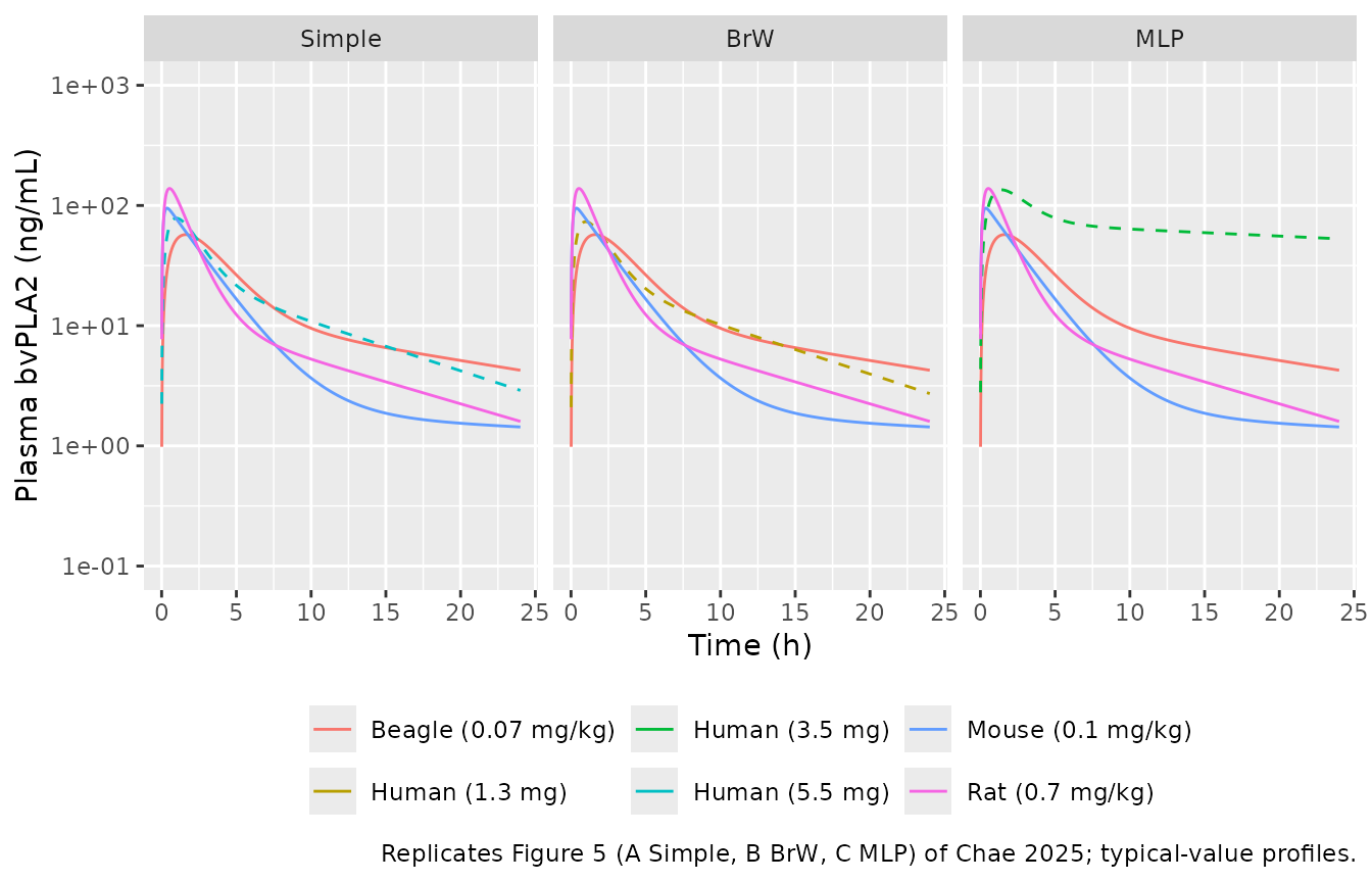
The Simple and BrW human curves match Figures 5A-B (peak near 75 ng/mL at 1 h, a few ng/mL at 24 h). The MLP curve does not match Figure 5C: see the next section.
human_nca_conc <- human_sim |>
  dplyr::filter(!is.na(Cc), time %in% c(0, 0.25, 0.5, 1, 1.5, 2, 3, 4, 6, 8, 10, 12, 16, 20, 24)) |>
  dplyr::mutate(id = 1L) |>
  dplyr::select(id, time, Cc, method)
human_dose <- data.frame(id = 1L, time = 0, amt = unname(human_doses), method = names(human_doses))
h_nca <- PKNCA::pk.nca(PKNCA::PKNCAdata(
  PKNCA::PKNCAconc(human_nca_conc, Cc ~ time | method + id),
  PKNCA::PKNCAdose(human_dose, amt ~ time | method + id),
  intervals = data.frame(start = 0, end = 24, cmax = TRUE, tmax = TRUE, auclast = TRUE, half.life = TRUE)
))
# Table 4 of Chae 2025; AUC converted from ug*h/mL to ng*h/mL.
published_t4 <- tibble::tribble(
  ~method, ~cmax, ~tmax, ~auclast, ~half.life,
  "Simple", 78.4, 1, 409, 7.39,
  "BrW", 73.3, 1, 382, 7.40,
  "MLP", 64.3, 0.5, 378, 3.35
)
cmp_t4 <- nlmixr2lib::ncaComparisonTable(
  simulated = h_nca,
  reference = published_t4,
  by = "method",
  units = c(cmax = "ng/mL", tmax = "h", auclast = "ng*h/mL", half.life = "h"),
  tolerance_pct = 20
)
knitr::kable(cmp_t4, caption = "Typical human profile vs. Table 4 of Chae 2025. * differs by more than 20%.")| NCA parameter | method | Reference | Simulated | % diff |
|---|---|---|---|---|
| Cmax (ng/mL) | Simple | 78.4 | 78.3 | -0.1% |
| Cmax (ng/mL) | BrW | 73.3 | 73.3 | +0.1% |
| Cmax (ng/mL) | MLP | 64.3 | 135 | +109.7%* |
| Tmax (h) | Simple | 1 | 1 | +0.0% |
| Tmax (h) | BrW | 1 | 1 | +0.0% |
| Tmax (h) | MLP | 0.5 | 1.5 | +200.0%* |
| AUClast (ng*h/mL) | Simple | 409 | 394 | -3.6% |
| AUClast (ng*h/mL) | BrW | 382 | 370 | -3.1% |
| AUClast (ng*h/mL) | MLP | 378 | 1670 | +341.9%* |
| t½ (h) | Simple | 7.39 | 7.35 | -0.5% |
| t½ (h) | BrW | 7.4 | 7.36 | -0.6% |
| t½ (h) | MLP | 3.35 | 52.8 | +1477.3%* |
# Terminal half-life from the disposition eigenvalue of each projection.
terminal_t12 <- function(cl, vc, vp, q) {
  k10 <- cl / vc
  k12 <- q / vc
  k21 <- q / vp
  s <- k10 + k12 + k21
  log(2) / ((s - sqrt(s^2 - 4 * k10 * k21)) / 2)
}
pk_of <- function(m) {
  th <- readModelDb(human_models[[m]])()$theta
  exp(th[c("lcl", "lvc", "lvp", "lq")])
}
t12 <- sapply(names(human_models), function(m) do.call(terminal_t12, as.list(unname(pk_of(m)))))
peak <- human_sim |>
  dplyr::group_by(method) |>
  dplyr::summarise(cmax = max(Cc), tmax = time[which.max(Cc)], .groups = "drop")
pk <- setNames(peak$cmax, peak$method)
tk <- setNames(peak$tmax, peak$method)
knitr::kable(data.frame(
  Method = names(t12),
  "Terminal t1/2 (h)" = unname(round(t12, 2)),
  "Cmax (ng/mL)" = unname(round(pk[names(t12)], 1)),
  "Tmax (h)" = unname(tk[names(t12)]),
  check.names = FALSE
), row.names = FALSE)| Method | Terminal t1/2 (h) | Cmax (ng/mL) | Tmax (h) |
|---|---|---|---|
| Simple | 7.39 | 78.3 | 0.99 |
| BrW | 7.39 | 73.4 | 0.99 |
| MLP | 53.12 | 135.0 | 1.42 |
# Deterministic typical-value solves: tight tolerances are appropriate.
stopifnot(
  abs(pk[["Simple"]] / 78.4 - 1) < 0.01,
  abs(pk[["BrW"]] / 73.3 - 1) < 0.01,
  abs(tk[["Simple"]] - 1) <= 0.05,
  abs(tk[["BrW"]] - 1) <= 0.05,
  abs(t12[["Simple"]] / 7.39 - 1) < 0.02,
  abs(t12[["BrW"]] / 7.40 - 1) < 0.02,
  # The printed MLP parameter set gives a terminal half-life an order of
  # magnitude longer than Table 4 -- the discrepancy documented below.
  t12[["MLP"]] > 40
)
The Simple and BrW projections reproduce Table 4 Cmax, Tmax and terminal half-life to within 1-2%. The PKNCA AUC to 24 h is about 3% below Table 4 for both; the eigenvalue (terminal) half-life in the second table and the PKNCA half-life over 0-24 h both match Table 4 to within 1%.
The MLP projection
The MLP file carries Table 3 as printed (CL/F 0.612 L/h, also stated in the Results text). That parameter set does not reproduce the paper’s own MLP simulation:
- With CL/F = 0.612 L/h the terminal half-life is about 53 h and the AUC to 24 h is about four times the Table 4 value (0.378 ug.h/mL); the 24 h concentration is ~50 ng/mL, whereas Figure 5C shows the human curve near 0.6 ng/mL at 24 h.
- Table 4 lists “CL/F 0.00917” for MLP. Read on the same scale as its Simple and BrW entries (0.01248 and 0.00316, i.e. one thousandth of the Table 3 L/h values) this is 9.17 L/h, consistent with dose / AUC = 3.5 / 0.378 = 9.26 L/h, and with the 3.5 mg dose back-calculated from the mouse target (0.397 x 9.17 = 3.6 mg).
- Even with CL/F = 9.17 L/h and the Table 3 volumes, no ka gives the Table 4 combination of Cmax 64.3 ng/mL at 0.5 h with a 3.35 h half-life, so the Table 4 MLP simulation used a parameter set that is not printed.
mlp_alt <- two_cmt_sd(0.803, 9.17, 10.0, 34.7, 7.59, 3.5)
knitr::kable(data.frame(
  "CL/F (L/h)" = c(0.612, 9.17),
  "Cmax (ng/mL)" = round(c(pk[["MLP"]], max(mlp_alt$c)), 1),
  "Tmax (h)" = c(tk[["MLP"]], mlp_alt$t[which.max(mlp_alt$c)]),
  "AUC0-24 (ug*h/mL)" = signif(c(
    trap(human_sim$time[human_sim$method == "MLP"], human_sim$Cc[human_sim$method == "MLP"]) / 1000,
    trap(mlp_alt$t, mlp_alt$c) / 1000
  ), 3),
  check.names = FALSE
), caption = "MLP projection with the Table 3 CL/F (shipped) and with the Table 4 CL/F read as 9.17 L/h (Table 4: Cmax 64.3 ng/mL, Tmax 0.5 h, AUC0-t 0.378 ug*h/mL).")| CL/F (L/h) | Cmax (ng/mL) | Tmax (h) | AUC0-24 (ug*h/mL) |
|---|---|---|---|
| 0.612 | 135.0 | 1.42 | 1.670 |
| 9.170 | 87.3 | 0.89 | 0.366 |
The maintainers ship the printed Table 3 parameters, which are the
paper’s stated projection, and flag the inconsistency here. To reproduce
the Table 4 MLP exposure approximately, override the clearance:
rxode2::ini(readModelDb("Chae_2025_beeVenomPLA2_human_mlp"), lcl = fixed(log(9.17))).
The paper’s recommended FIH projection is BrW (highest R2, FIH dose 1.3
mg), which is unaffected.
Assumptions and deviations
- Human ka. Not printed for any human projection. All three human files use the rat Table 2 estimate, 0.803 1/h (fixed), which reproduces the Table 4 Simple and BrW Cmax, Tmax and half-life (sweep above). This is a back-solved value, not a reported one.
- MLP clearance. The MLP file carries CL/F = 0.612 L/h from Table 3 and the Results text, which conflicts with Table 4 and Figure 5C (see above).
- Residual error. Methods describes a combined additive + proportional residual model, but Table 2 reports only a proportional term for each species, so the animal models carry proportional error only.
-
BSV. Reported as CV%; converted to log-normal
variances with
log(CV^2 + 1). Parameters without a reported BSV have none. - Units. The animal parameters are per kg (Table 2); the rat Vp/F is printed as “6.89 L” in the Results prose and as L/kg in Table 2, and the table unit is used. The Table 2 rat column header reads “0.2-0.5 mg/kg” while Methods, Table 1 and Figure 3 cover 0.2-2 mg/kg.
-
Human weight scaling. Only the simple-allometry
exponents are printed, so only
Chae_2025_beeVenomPLA2_human_simplescales withWT(reference 70 kg). The BrW and MLP regressions also depend on species brain weight or lifespan, whose values and coefficients are not printed; those two files encode the 70 kg prediction only. - Human projections are deterministic. They carry no between-subject variability, and the residual error is fixed to zero.
- Mouse efficacious AUC. The integration window of the reported 0.397 ug.h/mL is not stated; it lies between the typical mouse AUC to 24 h and to infinity.
- No erratum or correction notice for Chae 2025 was found as of 2026-11-09.