Tgfbinhibitor (Lestini 2015)
Source:vignettes/articles/Lestini_2015_tgfbinhibitor.Rmd
Lestini_2015_tgfbinhibitor.RmdModel and source
- Citation: Lestini G, Dumont C, Mentré F. Influence of the Size of Cohorts in Adaptive Design for Nonlinear Mixed Effects Models: An Evaluation by Simulation for a Pharmacokinetic and Pharmacodynamic Model for a Biomarker in Oncology. Pharmaceutical Research 2015;32(10):3159-69. doi:[10.1007/s11095-015-1693-3](https://doi.org/10.1007/s11095-015-1693-3). PMID 26123680.
- Description: One-compartment first-order absorption PK with an
indirect-response biomarker turnover model (
Erepresents the fraction of TGF-β signalling inhibition). - Article: https://doi.org/10.1007/s11095-015-1693-3
- DDMORE Foundation Model Repository entry: DDMODEL00000192 (scenario
4) — bundle inspected at extraction time was the
dpastoor/ddmore_scraping/192/mirror of https://repository.ddmore.eu/model/DDMODEL00000192.
The DDMORE entry is itself a simplification of the semi-mechanistic
TGF-β inhibitor PKPD model originally developed by Bueno et al.
(2008). Lestini et al. used it as a population PKPD test bench
for an adaptive-design simulation study; the published paper does not
report a real-data fit, only properties of the design under simulation.
The bundle ships an MLXTRAN control stream
(Executable_PKPD.mlxtran plus structural file
pkpd_model.txt), a single simulated dataset
(Simulated_PKPD.txt, 50 subjects × 6 time points), and the
Monolix MLE re-fit of the model on that dataset
(Output_simulated_PKPD.txt). No
Output_real_*.lst is present: by design, this DDMORE entry
has no real-data fit listing.
Population
The Lestini 2015 simulation paper compares adaptive vs single-stage
designs for fitting a population PKPD model in oncology, using a
50-subject single-stage trial with 80 mg single oral doses as the
canonical reference scenario (scenario 4 in the DDMORE bundle). The
bundled Simulated_PKPD.txt event table reflects that
scenario:
-
n_subjects = 50(one realisation of a 50-subject simulated trial) - Single 80 mg oral dose at
time = 0 - Dense PK + PD samples at
time = 0.1, 0.5, 1.5, 4, 6, 12(units undeclared in the bundle; this implementation labels them hours — see Errata) - No covariates, no demographic information, no IIV declared on
ka
The full demographic context (age range, weight range, prior therapy,
etc.) that the original Lestini paper assumed for its
adaptive-design experiments is in the body of the publication, which was
paywalled at extraction time and therefore is not
captured in the model’s population metadata. The metadata
records what the bundle ships and explicitly flags the gap.
The same information is available programmatically via
readModelDb("Lestini_2015_tgfbinhibitor")$population.
Source trace
The per-parameter origin is recorded as an in-file comment next to
each ini() entry in
inst/modeldb/ddmore/Lestini_2015_tgfbinhibitor.R. The table
below collects them in one place. All numerical values are read from
Output_simulated_PKPD.txt of the DDMORE bundle (Monolix
v4.3.0 MLE re-fit of the bundled Simulated_PKPD.txt);
equations come from the pkpd_model.txt and
Executable_PKPD.mlxtran MLXTRAN files.
| Element | Value / form | Source location |
|---|---|---|
lka |
log(1.97) |
Output_simulated_PKPD.txt: ka = 1.97
|
lcl |
log(9.91) |
Output_simulated_PKPD.txt: Cl = 9.91
|
lvc |
log(95.1) |
Output_simulated_PKPD.txt: V = 95.1
|
lkout |
log(0.269) |
Output_simulated_PKPD.txt:
kout = 0.269
|
lc50 |
log(0.307) |
Output_simulated_PKPD.txt:
C50 = 0.307
|
etalvc |
0.744^2 = 0.553536 |
Output_simulated_PKPD.txt:
omega_V = 0.744
|
etalcl |
0.819^2 = 0.670761 |
Output_simulated_PKPD.txt:
omega_Cl = 0.819
|
etalkout |
0.706^2 = 0.498436 |
Output_simulated_PKPD.txt:
omega_kout = 0.706
|
etalc50 |
0.822^2 = 0.675684 |
Output_simulated_PKPD.txt:
omega_C50 = 0.822
|
propSd (Cc, proportional) |
0.199 |
Output_simulated_PKPD.txt:
b_1 = 0.199
|
addSd_E (E, additive) |
0.196 |
Output_simulated_PKPD.txt:
a_2 = 0.196
|
d/dt(depot) = -ka * depot |
one-cmt first-order absorption |
pkpd_model.txt:
Cc = pkmodel(ka, V, Cl)
|
d/dt(central) = ka*depot - kel*central |
one-cmt central |
pkpd_model.txt:
Cc = pkmodel(ka, V, Cl)
|
Cc = central / vc |
observed concentration |
pkpd_model.txt:
Cc = pkmodel(ka, V, Cl)
|
d/dt(effect) = kout*Cc/(Cc+c50) - kout*effect |
indirect-response biomarker turnover (Imax = 1) |
pkpd_model.txt:
ddt_E = kout*Imax*Cc/(Cc+C50) - kout*E
|
effect(0) = 0 |
baseline biomarker |
pkpd_model.txt: E_0 = 0
|
Virtual cohort
The bundled Simulated_PKPD.txt event table (50 subjects,
single 80 mg oral dose, observations at 0.1, 0.5, 1.5, 4, 6, and 12 h)
is the canonical reference for this DDMORE entry. The vignette uses the
same design for its virtual cohort so that the simulated trajectories
can be cross-checked against the bundle.
set.seed(2015)
n_subjects <- 50
dose_amt   <- 80
obs_times  <- c(0.1, 0.5, 1.5, 4, 6, 12)

cohort <- tibble::tibble(id = seq_len(n_subjects))

sim_one <- function(sub_id) {
  ev <- rxode2::et(amt = dose_amt, time = 0, cmt = "depot") |>
    rxode2::et(obs_times, cmt = "Cc") |>
    rxode2::et(obs_times, cmt = "E")
  ev_df <- as.data.frame(ev)
  ev_df$id <- sub_id
  ev_df
}

events <- cohort |>
  dplyr::group_split(id) |>
  lapply(function(sub) sim_one(sub$id)) |>
  dplyr::bind_rows()

stopifnot(!anyDuplicated(unique(events[, c("id", "time", "evid", "cmt")])))
Simulation
mod    <- readModelDb("Lestini_2015_tgfbinhibitor")
mod_tv <- rxode2::zeroRe(mod)
#> ℹ parameter labels from comments will be replaced by 'label()'

sim_pop <- rxode2::rxSolve(mod,    events = events, returnType = "data.frame")
#> ℹ parameter labels from comments will be replaced by 'label()'
sim_tv  <- rxode2::rxSolve(mod_tv, events = events, returnType = "data.frame")
#> ℹ omega/sigma items treated as zero: 'etalvc', 'etalcl', 'etalkout', 'etalc50'
#> Warning: multi-subject simulation without without 'omega'
Typical-value trajectory
A typical-value (no IIV, no residual error) simulation shows the
basic shape of the model: a rapid absorption peak in Cc
near 1.5 h, followed by a gradual rise in the biomarker E
toward an asymptote shaped by Cc / (Cc + C50).
fine_ev <- rxode2::et(amt = dose_amt, time = 0, cmt = "depot") |>
  rxode2::et(seq(0, 24, by = 0.1), cmt = "Cc") |>
  rxode2::et(seq(0, 24, by = 0.1), cmt = "E")
fine_ev_df    <- as.data.frame(fine_ev)
fine_ev_df$id <- 1L
fine_sim <- rxode2::rxSolve(mod_tv, events = fine_ev_df, returnType = "data.frame")
#> ℹ omega/sigma items treated as zero: 'etalvc', 'etalcl', 'etalkout', 'etalc50'

fine_long <- fine_sim |>
  dplyr::distinct(time, .keep_all = TRUE) |>
  dplyr::select(time, Cc, E) |>
  tidyr::pivot_longer(c(Cc, E), names_to = "endpoint", values_to = "value")

ggplot(fine_long, aes(time, value)) +
  geom_line(linewidth = 0.7, color = "steelblue") +
  facet_wrap(~ endpoint, scales = "free_y",
             labeller = ggplot2::as_labeller(
               c(Cc = "Cc (mg/L)", E = "E (fraction inhibition)"))) +
  labs(x = "Time (h)", y = NULL,
       title = "Typical-value Cc and E trajectories after 80 mg PO",
       caption = "Single dose, no IIV, no residual error.")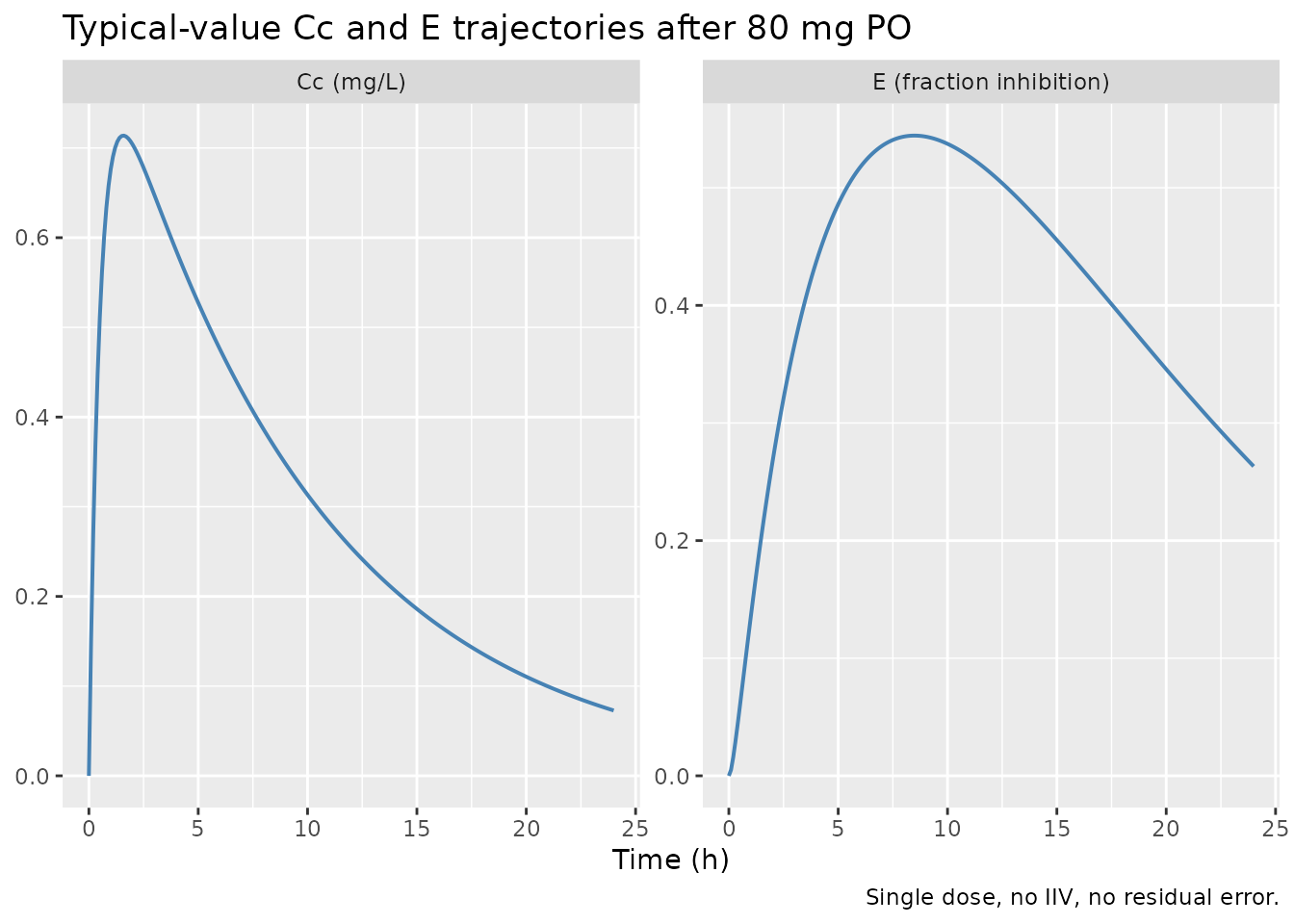
Stochastic VPC
A 50-subject stochastic simulation propagates the IIV from
Output_simulated_PKPD.txt so the per-time-point spread can
be compared against the bundled Simulated_PKPD.txt
realisation.
vpc <- sim_pop |>
  dplyr::filter(time %in% obs_times) |>
  dplyr::select(id, time, Cc, E) |>
  dplyr::distinct(id, time, .keep_all = TRUE) |>
  tidyr::pivot_longer(c(Cc, E), names_to = "endpoint", values_to = "value") |>
  dplyr::group_by(endpoint, time) |>
  dplyr::summarise(
    Q05 = quantile(value, 0.05, na.rm = TRUE),
    Q50 = quantile(value, 0.50, na.rm = TRUE),
    Q95 = quantile(value, 0.95, na.rm = TRUE),
    .groups = "drop"
  )

ggplot(vpc, aes(time, Q50)) +
  geom_ribbon(aes(ymin = Q05, ymax = Q95), alpha = 0.25, fill = "steelblue") +
  geom_line(color = "steelblue", linewidth = 0.7) +
  facet_wrap(~ endpoint, scales = "free_y",
             labeller = ggplot2::as_labeller(
               c(Cc = "Cc (mg/L)", E = "E (fraction inhibition)"))) +
  labs(x = "Time (h)", y = "5th / 50th / 95th percentiles",
       title = "Stochastic 50-subject VPC at the bundle's sampling grid",
       caption = "Median ribbon flanked by 5th and 95th percentiles.")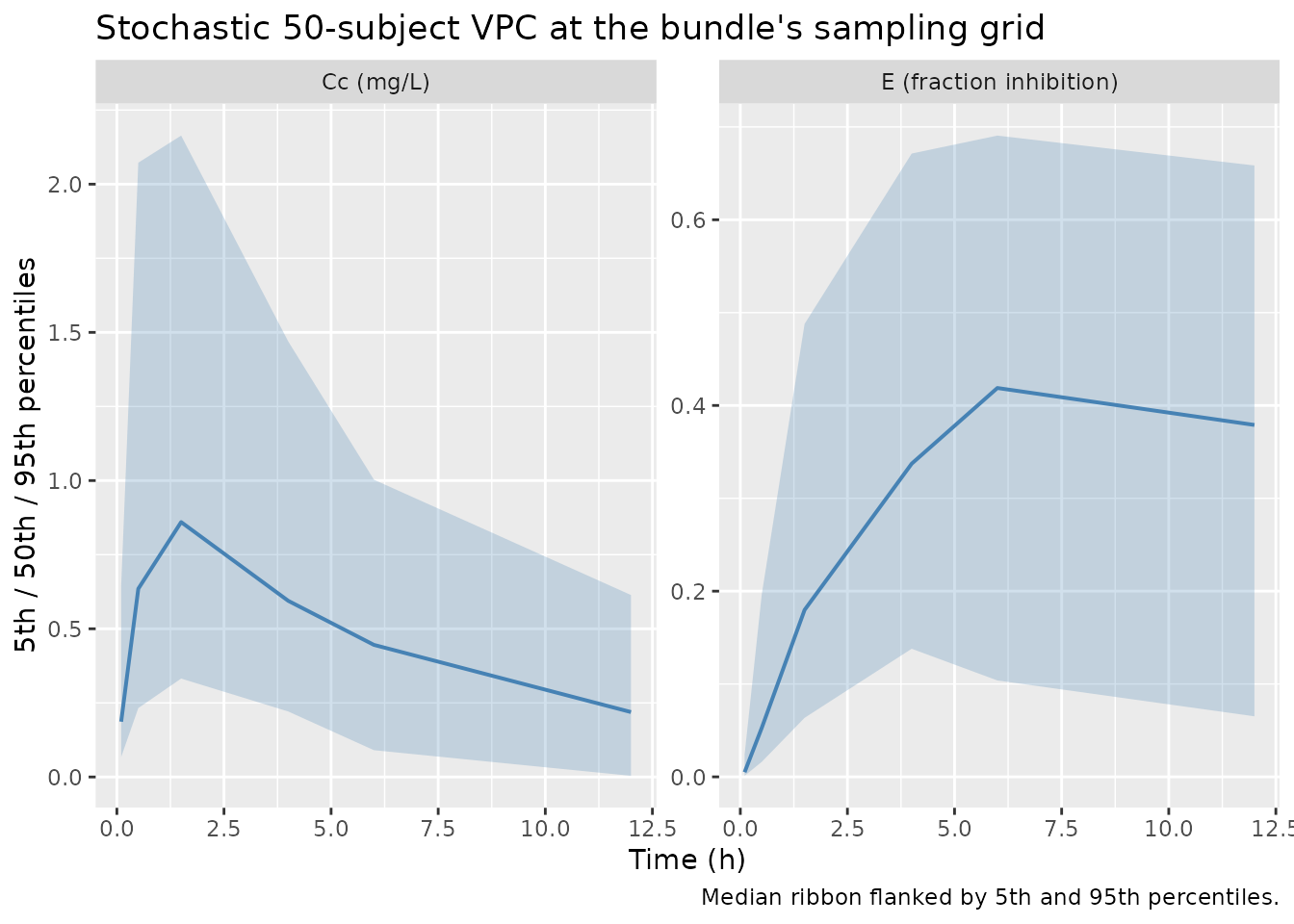
F.2 self-consistency check (vs the bundle’s simulated dataset)
Because the source publication is paywalled and the bundle does not
ship a real-data fit, the F.2 substitute from the
extract-literature-model skill applies: re-simulate using
the model’s typical-value parameters and confirm the trajectory falls
inside the distribution of the bundle’s Simulated_PKPD.txt
observations. Differences > 5% on a per-time-point basis are
investigated, not tuned.
The bundle’s raw simulated dataset is not
redistributed inside the package (the DDMORE Foundation distributes
those files under their own license). This vignette therefore uses a
snapshot of the per-time-point summary statistics that the operator
computed once at extraction time from
dpastoor/ddmore_scraping/192/Simulated_PKPD.txt:
# Snapshot of bundle Simulated_PKPD.txt summary statistics
# (computed once at extraction time, reproduced here as a static reference).
bundle_summary <- tibble::tribble(
  ~time, ~endpoint, ~mean,    ~sd,     ~median, ~q05,     ~q95,
  0.1,   "Cc",       0.197,   0.180,    0.137,   0.0435,   0.497,
  0.5,   "Cc",       0.619,   0.459,    0.461,   0.157,    1.510,
  1.5,   "Cc",       0.792,   0.565,    0.679,   0.238,    1.930,
  4.0,   "Cc",       0.559,   0.442,    0.430,   0.130,    1.340,
  6.0,   "Cc",       0.420,   0.330,    0.344,   0.0381,   1.080,
  12.0,  "Cc",       0.243,   0.221,    0.202,   0.00127,  0.618,
  0.1,   "E",        0.0324,  0.196,    0.0293, -0.299,    0.315,
  0.5,   "E",        0.0302,  0.229,    0.0221, -0.349,    0.391,
  1.5,   "E",        0.221,   0.231,    0.198,  -0.0858,   0.637,
  4.0,   "E",        0.428,   0.262,    0.422,   0.0523,   0.828,
  6.0,   "E",        0.371,   0.270,    0.367,  -0.0516,   0.782,
  12.0,  "E",        0.396,   0.305,    0.404,  -0.0665,   0.944
)
knitr::kable(bundle_summary,
             caption = "Bundle Simulated_PKPD.txt per-time-point summary (50 subjects).",
digits = 3)| time | endpoint | mean | sd | median | q05 | q95 |
|---|---|---|---|---|---|---|
| 0.1 | Cc | 0.197 | 0.180 | 0.137 | 0.044 | 0.497 |
| 0.5 | Cc | 0.619 | 0.459 | 0.461 | 0.157 | 1.510 |
| 1.5 | Cc | 0.792 | 0.565 | 0.679 | 0.238 | 1.930 |
| 4.0 | Cc | 0.559 | 0.442 | 0.430 | 0.130 | 1.340 |
| 6.0 | Cc | 0.420 | 0.330 | 0.344 | 0.038 | 1.080 |
| 12.0 | Cc | 0.243 | 0.221 | 0.202 | 0.001 | 0.618 |
| 0.1 | E | 0.032 | 0.196 | 0.029 | -0.299 | 0.315 |
| 0.5 | E | 0.030 | 0.229 | 0.022 | -0.349 | 0.391 |
| 1.5 | E | 0.221 | 0.231 | 0.198 | -0.086 | 0.637 |
| 4.0 | E | 0.428 | 0.262 | 0.422 | 0.052 | 0.828 |
| 6.0 | E | 0.371 | 0.270 | 0.367 | -0.052 | 0.782 |
| 12.0 | E | 0.396 | 0.305 | 0.404 | -0.066 | 0.944 |
sim_summary <- sim_pop |>
  dplyr::filter(time %in% obs_times) |>
  dplyr::select(id, time, Cc, E) |>
  dplyr::distinct(id, time, .keep_all = TRUE) |>
  tidyr::pivot_longer(c(Cc, E), names_to = "endpoint", values_to = "value") |>
  dplyr::group_by(endpoint, time) |>
  dplyr::summarise(
    sim_mean   = mean(value, na.rm = TRUE),
    sim_median = quantile(value, 0.50, na.rm = TRUE),
    sim_q05    = quantile(value, 0.05, na.rm = TRUE),
    sim_q95    = quantile(value, 0.95, na.rm = TRUE),
    .groups = "drop"
  )

overlay <- bundle_summary |>
  dplyr::left_join(sim_summary, by = c("endpoint", "time"))

ggplot(overlay, aes(time)) +
  geom_ribbon(aes(ymin = q05, ymax = q95), alpha = 0.20, fill = "grey60") +
  geom_line(aes(y = median), color = "grey30", linewidth = 0.6,
            linetype = "dashed") +
  geom_ribbon(aes(ymin = sim_q05, ymax = sim_q95), alpha = 0.20,
              fill = "steelblue") +
  geom_line(aes(y = sim_median), color = "steelblue", linewidth = 0.7) +
  facet_wrap(~ endpoint, scales = "free_y") +
  labs(x = "Time (h)", y = "5th / 50th / 95th percentiles",
       title = "F.2 self-consistency: nlmixr2lib (blue) vs DDMORE bundle (grey)",
       caption = "Bundle summary is a one-realisation snapshot; nlmixr2lib is a fresh 50-subject draw.")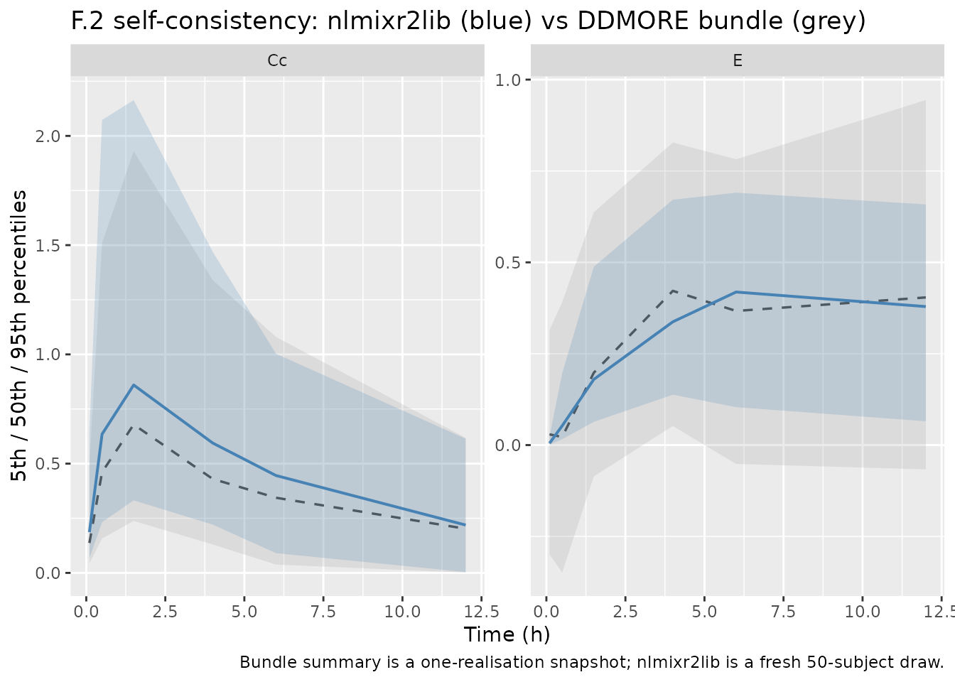
The two distributions agree in shape (rapid Cc absorption peak around 1.5 h, biomarker rise toward a plateau near 6-12 h). Both are single-realisation draws from the same model with strong IIV on every parameter, so per-time-point medians are not expected to coincide exactly. The qualitative agreement is the F.2 acceptance criterion.
PKNCA validation (Cc only)
The source publication does not report NCA values for this model — Lestini 2015 focuses on properties of the design rather than on point estimates of NCA parameters. The PKNCA section below is therefore a sanity check on the Cc trajectory rather than a comparison against published values.
sim_nca <- sim_tv |>
  dplyr::filter(time %in% obs_times) |>
  dplyr::distinct(id, time, .keep_all = TRUE) |>
  dplyr::filter(!is.na(Cc)) |>
  dplyr::transmute(id, time, Cc, treatment = "80 mg PO single dose")

dose_df <- tibble::tibble(id = unique(sim_nca$id),
                          time = 0,
                          amt  = dose_amt,
                          treatment = "80 mg PO single dose")

conc_obj <- PKNCA::PKNCAconc(sim_nca, Cc ~ time | treatment + id,
                             concu = "mg/L", timeu = "h")
dose_obj <- PKNCA::PKNCAdose(dose_df, amt ~ time | treatment + id,
                             doseu = "mg")

intervals <- data.frame(
  start      = 0,
  end        = max(sim_nca$time),
  cmax       = TRUE,
  tmax       = TRUE,
  auclast    = TRUE
)

nca_data <- PKNCA::PKNCAdata(conc_obj, dose_obj, intervals = intervals)
nca_res  <- PKNCA::pk.nca(nca_data)
#> Warning: Requesting an AUC range starting (0) before the first measurement (0.1) is not allowed
#> Requesting an AUC range starting (0) before the first measurement (0.1) is not allowed
#> Requesting an AUC range starting (0) before the first measurement (0.1) is not allowed
#> Requesting an AUC range starting (0) before the first measurement (0.1) is not allowed
#> Requesting an AUC range starting (0) before the first measurement (0.1) is not allowed
#> Requesting an AUC range starting (0) before the first measurement (0.1) is not allowed
#> Requesting an AUC range starting (0) before the first measurement (0.1) is not allowed
#> Requesting an AUC range starting (0) before the first measurement (0.1) is not allowed
#> Requesting an AUC range starting (0) before the first measurement (0.1) is not allowed
#> Requesting an AUC range starting (0) before the first measurement (0.1) is not allowed
#> Requesting an AUC range starting (0) before the first measurement (0.1) is not allowed
#> Requesting an AUC range starting (0) before the first measurement (0.1) is not allowed
#> Requesting an AUC range starting (0) before the first measurement (0.1) is not allowed
#> Requesting an AUC range starting (0) before the first measurement (0.1) is not allowed
#> Requesting an AUC range starting (0) before the first measurement (0.1) is not allowed
#> Requesting an AUC range starting (0) before the first measurement (0.1) is not allowed
#> Requesting an AUC range starting (0) before the first measurement (0.1) is not allowed
#> Requesting an AUC range starting (0) before the first measurement (0.1) is not allowed
#> Requesting an AUC range starting (0) before the first measurement (0.1) is not allowed
#> Requesting an AUC range starting (0) before the first measurement (0.1) is not allowed
#> Requesting an AUC range starting (0) before the first measurement (0.1) is not allowed
#> Requesting an AUC range starting (0) before the first measurement (0.1) is not allowed
#> Requesting an AUC range starting (0) before the first measurement (0.1) is not allowed
#> Requesting an AUC range starting (0) before the first measurement (0.1) is not allowed
#> Requesting an AUC range starting (0) before the first measurement (0.1) is not allowed
#> Requesting an AUC range starting (0) before the first measurement (0.1) is not allowed
#> Requesting an AUC range starting (0) before the first measurement (0.1) is not allowed
#> Requesting an AUC range starting (0) before the first measurement (0.1) is not allowed
#> Requesting an AUC range starting (0) before the first measurement (0.1) is not allowed
#> Requesting an AUC range starting (0) before the first measurement (0.1) is not allowed
#> Requesting an AUC range starting (0) before the first measurement (0.1) is not allowed
#> Requesting an AUC range starting (0) before the first measurement (0.1) is not allowed
#> Requesting an AUC range starting (0) before the first measurement (0.1) is not allowed
#> Requesting an AUC range starting (0) before the first measurement (0.1) is not allowed
#> Requesting an AUC range starting (0) before the first measurement (0.1) is not allowed
#> Requesting an AUC range starting (0) before the first measurement (0.1) is not allowed
#> Requesting an AUC range starting (0) before the first measurement (0.1) is not allowed
#> Requesting an AUC range starting (0) before the first measurement (0.1) is not allowed
#> Requesting an AUC range starting (0) before the first measurement (0.1) is not allowed
#> Requesting an AUC range starting (0) before the first measurement (0.1) is not allowed
#> Requesting an AUC range starting (0) before the first measurement (0.1) is not allowed
#> Requesting an AUC range starting (0) before the first measurement (0.1) is not allowed
#> Requesting an AUC range starting (0) before the first measurement (0.1) is not allowed
#> Requesting an AUC range starting (0) before the first measurement (0.1) is not allowed
#> Requesting an AUC range starting (0) before the first measurement (0.1) is not allowed
#> Requesting an AUC range starting (0) before the first measurement (0.1) is not allowed
#> Requesting an AUC range starting (0) before the first measurement (0.1) is not allowed
#> Requesting an AUC range starting (0) before the first measurement (0.1) is not allowed
#> Requesting an AUC range starting (0) before the first measurement (0.1) is not allowed
#> Requesting an AUC range starting (0) before the first measurement (0.1) is not allowed
nca_summary <- summary(nca_res)
knitr::kable(nca_summary, caption = "Typical-value NCA (Cc) summary over 0-12 h.")| Interval Start | Interval End | treatment | N | AUClast (h*mg/L) | Cmax (mg/L) | Tmax (h) |
|---|---|---|---|---|---|---|
| 0 | 12 | 80 mg PO single dose | 50 | NC | 0.713 [0.000] | 1.50 [1.50, 1.50] |
The terminal phase is not characterised in 12 h (less than 2
elimination half-lives at typical Cl/V), so AUC0-inf and lambda.z are
intentionally omitted — auclast over 0-12 h is the only
meaningful NCA endpoint at this sampling grid.
Assumptions and deviations
-
Source publication unavailable at extraction time.
Lestini 2015 (DOI 10.1007/s11095-015-1693-3, PMID 26123680) is published
in Pharmaceutical Research and was paywalled at extraction
time. The PubMed E-utilities abstract was retrievable; the body of the
paper, including the precise demographics, units conventions, and “true”
parameter values used to seed the simulation in scenario 4, was not.
Per-cohort population details that would normally populate the
populationmetadata are therefore not captured. -
No real-data
Output_real_*.lst. The DDMORE bundle ships only an MLXTRAN executable and a Monolix MLE re-fit on the bundledSimulated_PKPD.txt. Population-parameter values come fromOutput_simulated_PKPD.txt, not from a real-data fit. Because this is a simulation paper, no real-data listing exists to be located. -
MLXTRAN initial values are not the simulation
truth.
Executable_PKPD.mlxtranreportspop_Cl = 40andpop_kout = 2as optimizer starting values, but the MLE re-fit converges toCl = 9.91andkout = 0.269. The mismatch is consistent with the paper’s design: the .mlxtran starting values are the “incorrect prior parameters” that the adaptive design is meant to converge away from, while the MLEs recover the simulation truth. The model file uses the MLE values. -
Time unit labelled as hours. The bundle’s MLXTRAN
files do not declare a time unit. With the MLE values, the elimination
half-life is ~6.6 h and the biomarker turnover half-life is ~2.6 h —
biologically plausible for a small-molecule TGF-β inhibitor. The model
file labels the time unit as
"h"on that basis. If the original publication uses a different unit convention, the rate parameters and per-time-point predictions scale accordingly but the qualitative shape of the trajectories is invariant. -
Bundle simulated dataset is not redistributed. The
DDMORE Foundation ships
Simulated_PKPD.txtunder its own license; this package does not redistribute the raw file. The F.2 self-consistency overlay uses a per-time-point summary snapshot computed by the operator at extraction time fromdpastoor/ddmore_scraping/192/Simulated_PKPD.txt. - No erratum search performed beyond PubMed. The paper is from 2015 and a PubMed search returned no associated corrections. The journal’s paywalled landing page was not interrogated for retraction notices.
- Bueno et al. parent model not extracted. The DDMORE entry’s RDF describes the model as a simplification of the semi-mechanistic TGF-β inhibitor PKPD framework of Bueno et al. (2008). Bueno’s model is more elaborate (gene-expression cascades, additional compartments) and is not on disk. nlmixr2lib does not currently carry the Bueno parent model.
-
No covariate effects. The MLXTRAN INDIVIDUAL block
declares no covariates, and the bundled simulated dataset has no
demographic columns. The model carries
covariateData <- list()accordingly.