Iohexol + creatinine joint GFR / OCT2-MATE model (Chen 2025) • nlmixr2lib

Model and source

Citation: Chen Z, Dong Q, Dokos C, Boland J, Fuhr U, Taubert M. A Joint Pharmacometric Model of Iohexol and Creatinine Administered through a Meat Meal to Assess GFR and Renal OCT2/MATE Activity. Clin Pharmacol Ther. 2025;118(2):510-520. doi:10.1002/cpt.3612. Parameter values are taken from Table 3 and from the deposited NONMEM control stream in the Supporting Information (CPT-118-510-s001.docx), which is the authoritative source wherever the two disagree; see the validation vignette Errata.
Description: Joint population pharmacokinetic model of intravenous iohexol and creatinine in 14 healthy adults (Chen 2025), fit simultaneously to dense plasma and urine data for both analytes. Iohexol follows three-compartment linear disposition and its clearance IS the glomerular filtration rate (GFR). Creatinine follows one-compartment disposition driven by two inputs: a zero-order endogenous generation rate (CGR, replaced during model development by the Cockcroft-Gault expression in age, total body weight and sex) and first-order absorption of a cooked-beef creatinine load with a lag time and an estimated bioavailability. Creatinine clearance is the sum of GFR and a net tubular secretion arm (nCTS), the OCT2/MATE-mediated secretory flux net of tubular reabsorption, which accounted for 31% of total creatinine clearance in this cohort. Both analytes are assumed to be solely renally eliminated, so each carries a cumulative urinary-excretion state and a urine output alongside its plasma output. A piecewise-sine circadian rhythm (14 h daytime rise, 10 h nocturnal fall) multiplies GFR and nCTS with a single shared pair of amplitudes. All clearances and volumes are allometrically scaled to a 70 kg reference weight with fixed exponents of 0.75 and 1.
Article: https://doi.org/10.1002/cpt.3612
Supplement (bioanalysis, NCA methods, Tables S1-S3, Figures S1-S8, and the full NONMEM control stream): https://doi.org/10.1002/cpt.3612 Supporting Information, file CPT-118-510-s001.docx
PubMed Central: https://www.ncbi.nlm.nih.gov/pmc/articles/PMC12272311/

Chen and colleagues gave 14 healthy volunteers intravenous iohexol as a reference glomerular filtration rate (GFR) probe and, in one study period, a 250 g cooked-beef meal as an oral creatinine load. Dense plasma and urine sampling of both analytes was fit simultaneously in a single joint model, which lets creatinine clearance be split into the part explained by filtration (pinned by iohexol) and the remainder, the net creatinine tubular secretion (nCTS) mediated by OCT2 and MATE1 / MATE2-K. The meal perturbs creatinine away from its steady-state baseline, which is what makes the creatinine volume of distribution identifiable: the paper’s headline results are a creatinine Vd of 41.3% of total body weight (well below the 60% commonly assumed) and an nCTS fraction of 31% of total creatinine clearance.

This is a single jointly-fit model, so it is packaged as one model file: inst/modeldb/specificDrugs/Chen_2025_iohexol_creatinine.R. Table 1 of the paper lists six creatinine dose / F1 / Vd settings; those are a model-selection ladder, not independent models, and setting 6 (estimate both F1 and Vd) is the one carried into the joint fit.

Population

Study population (Chen 2025 Table 2). Available programmatically as `rxode2::rxode(readModelDb('Chen_2025_iohexol_creatinine'))$population`.
Field	Value
Species	human
N subjects	14
N studies	2
N observations	2475
Age	23-48 years
Weight	59.1-95.8 kg
Female	35.7%
Disease state	Healthy volunteers with normal renal function (mean estimated GFR 102 mL/min/1.73 m^2, range 80-116)
Doses	Iohexol 259 mg or 3,235 mg as a single intravenous dose; creatinine administered as 250 g cooked beef (mean creatinine content 401 mg) eaten 25 minutes after the iohexol dose
Region	Germany (single centre, Cologne)

Fourteen healthy Caucasian volunteers (9 male, 5 female; two in a pilot study and twelve in the main study) were enrolled at a single centre in Cologne, Germany. Mean age was 33 years (range 23-48), mean total body weight 78.5 kg (59.1-95.8), mean height 178 cm, mean body mass index 24.7 kg/m^2, mean plasma albumin 45.6 g/L and mean screening plasma creatinine 0.90 mg/dL. Mean estimated GFR was 102 mL/min/1.73 m^2 (80-116), so the model was informed entirely by normal renal function. The dataset comprised 771 iohexol and 826 creatinine plasma concentrations plus 439 urine measurements for each analyte.

The crossover design had three periods: a reference period (3,235 mg iohexol, fasting), a test period (259 mg iohexol, fasting) and a meat period (3,235 mg iohexol plus 250 g cooked beef, mean creatinine content 401 mg, eaten 25 minutes after the iohexol dose). Washout was at least 7 days. Participants drank about 240 mL of water at each urine collection interval, which the Discussion notes may have kept them rehydrated and so contributed to the relatively high nCTS fraction.

Source trace

Every ini() entry in the model file carries an in-file comment naming its source. The table below collects them. Where Table 3 and the deposited NONMEM control stream disagree, the control stream is authoritative (see Assumptions and deviations).

Equation / parameter	Value	Source location
`lcl` (GFR = iohexol CL)	`log(5.22317)` L/h	Control stream `$THETA 7`; Table 3 “GFR (mL/min)” = 87.0
`lvc`	`log(8.69091)` L	`$THETA 8`; Table 3 “Vc (L)” = 8.69
`lq`	`log(0.130821)` L/h	`$THETA 9`; Table 3 “Qp1 (L/h)” = 0.131
`lvp`	`log(1.15193)` L	`$THETA 10`; Table 3 “Vp1 (L)” = 1.15
`lq2`	`log(4.00936)` L/h	`$THETA 11`; Table 3 “Qp2 (L/h)” = 4.01
`lvp2`	`log(4.21713)` L	`$THETA 12`; Table 3 “Vp2 (L)” = 4.22
`lka_creatinine`	`log(1.70996)` 1/h	`$THETA 1`; Table 3 “Ka (1/h)” = 1.71
`lcl_tsnet_creatinine` (nCTS)	`log(2.38177)` L/h	`$THETA 2`; Table 3 “nCTS (mL/min)” = 39.7
`lvc_creatinine` (creatinine Vd)	`log(28.943)` L	`$THETA 3`; Table 3 “Vd (L)” = 28.9
`lfdepot_creatinine` (F1)	`log(0.523045)`	`$THETA 4`; Table 3 “F1 (%)” = 52.3
`ltlag_creatinine`	`log(0.291197)` h	`$THETA 6`; Table 3 “Lag time (h)” = 0.291
`lksyn_creatinine` (CGR multiplier)	`fixed(log(1))`	`$THETA 5` = `1 FIX`; Table 3 CGR row prints the Cockcroft-Gault formula
`e_wt_cl`	`fixed(0.75)`	Table 3 “TBW on GFR, Qp1, Qp2, and nCTS” = 0.75 FIX; `TBWonCL`
`e_wt_vc`	`fixed(1)`	Methods “Covariate model”; `TBWonV`. See Errata on Table 3’s row label
`e_sexf_cl_tsnet_creatinine`	0.628122	`$THETA 15`; Table 3 “SEX on CTS” = 0.627
`cl_circ_famp_day`	0.0370398	`$THETA 13`; Table 3 “Circadian rhythm during daytime (%)” = 3.70
`cl_circ_famp_night`	0.0842088	`$THETA 14`; Table 3 “Circadian rhythm during nighttime (%)” = 8.42
IIV variances (8 etas)	see `ini()`	Control stream `$OMEGA`; cross-checked against Table 3’s CV(%) column
Residual SDs (4 proportional)	see `ini()`	Control stream `$SIGMA`; Table 3 “Random effect (RV)” rows
Creatinine generation rate `cg`	Cockcroft-Gault	Table 3 CGR row; control stream `CG=((140-AGE)TBW/72)(0.85*(1-SEX))60/100`
Circadian rhythm equation	n/a	Methods “Covariate model” printed equation; polarity and windows from control stream `$PK`
Allometric equation	n/a	Methods “Covariate model”; continuous-covariate form `Pi = PTV * (Cij / mean(Cj))^theta`
Categorical covariate form	n/a	Methods “Covariate model” equation (2), `Pi = PTV * theta^Cij`
Iohexol 3-compartment ODEs	n/a	Control stream `$DES`, `$MODEL NCOMP=7`; Figure S2 schematic
Creatinine 1-compartment ODEs + urine states	n/a	Control stream `$DES`; Figure S2 schematic
Creatinine steady-state initial condition	n/a	Control stream `$PK`: `C0 = CGR/CL_CRE`, `A_0(2) = C0*V_CRE`

Structural checks

Before simulating a cohort, confirm the packaged model reproduces the typical-value quantities the paper states in prose. Random effects are zeroed so these are exact typical-value predictions at the cohort mean covariates (78.5 kg, 33 years, male).

mod_typ <- rxode2::zeroRe(readModelDb("Chen_2025_iohexol_creatinine"))
#> ℹ parameter labels from comments will be replaced by 'label()'

typ_ev <- data.frame(
  id = 1L, time = seq(0, 48, by = 0.1), evid = 0L, amt = NA_real_,
  cmt = "central", dvid = 1L, WT = 78.5, AGE = 33, SEXF = 0
)
typ <- rxode2::rxSolve(mod_typ, typ_ev, useLinCmt = FALSE, returnType = "data.frame")
#> ℹ omega/sigma items treated as zero: 'etalcl', 'etalvc', 'etalvp', 'etalvp2', 'etalcl_tsnet_creatinine', 'etalvc_creatinine', 'etalksyn_creatinine', 'etalfdepot_creatinine'

gfr_mlmin   <- typ$cl[1] * 1000 / 60                       # cir == 1 exactly at t = 0
ncts_mlmin  <- typ$cl_tsnet_creatinine[1] * 1000 / 60
crcl_mlmin  <- gfr_mlmin + ncts_mlmin
ncts_frac   <- 100 * ncts_mlmin / crcl_mlmin
vd_pct_tbw  <- 100 * typ$vc_creatinine[1] / 78.5
cir_lo      <- min(typ$cir)
cir_hi      <- max(typ$cir)

checks <- tibble::tibble(
  Quantity = c("GFR at 78.5 kg (mL/min)", "Creatinine clearance at 78.5 kg (mL/min)",
               "nCTS share of creatinine clearance (%)", "Creatinine Vd (% of total body weight)",
               "Circadian trough (% of typical value)", "Circadian peak (% of typical value)"),
  Published = c(94.8, 138, 31, 41.3, 91.6, 104),
  Simulated = c(gfr_mlmin, crcl_mlmin, ncts_frac, vd_pct_tbw, 100 * cir_lo, 100 * cir_hi),
  Source = c("Results, popPK analysis", "Results, popPK analysis", "Results, popPK analysis",
             "Results / Abstract", "Results, popPK analysis", "Results, popPK analysis")
) |>
  mutate(`% diff` = 100 * (Simulated - Published) / Published)

knitr::kable(checks, digits = c(0, 1, 2, 0, 2), caption = "Typical-value structural checks against values stated in the text of Chen 2025.")

Typical-value structural checks against values stated in the text of Chen 2025.
Quantity	Published	Simulated	Source	% diff
GFR at 78.5 kg (mL/min)	94.8	94.87	Results, popPK analysis	0.07
Creatinine clearance at 78.5 kg (mL/min)	138.0	138.13	Results, popPK analysis	0.09
nCTS share of creatinine clearance (%)	31.0	31.32	Results, popPK analysis	1.03
Creatinine Vd (% of total body weight)	41.3	41.35	Results / Abstract	0.11
Circadian trough (% of typical value)	91.6	91.58	Results, popPK analysis	-0.02
Circadian peak (% of typical value)	104.0	103.70	Results, popPK analysis	-0.28


stopifnot(
  abs(gfr_mlmin  -  94.8) <  0.5,
  abs(crcl_mlmin - 138.0) <  1.0,
  abs(ncts_frac  -  31.0) <  0.5,
  abs(vd_pct_tbw -  41.3) <  0.1,
  abs(100 * cir_lo -  91.6) < 0.1,
  abs(100 * cir_hi - 104.0) < 0.4
)

Two further identities the model must satisfy exactly. First, iohexol is assumed to be eliminated solely by the kidney, so the drug in the three disposition compartments plus the cumulative urinary amount must always sum to the dose. Second, creatinine starts at, and in the absence of a meal stays at, its endogenous steady state CGR / CrCL, so the amount excreted over 24 h must equal 24 h worth of generation.

iox_ev <- data.frame(id = 1L, time = c(0, seq(0, 48, by = 0.1)), evid = c(1L, rep(0L, 481)),
                     amt = c(259, rep(NA_real_, 481)), cmt = "central",
                     dvid = c(NA_integer_, rep(1L, 481)), WT = 78.5, AGE = 33, SEXF = 0)
iox <- rxode2::rxSolve(mod_typ, iox_ev, useLinCmt = FALSE, returnType = "data.frame")
#> ℹ omega/sigma items treated as zero: 'etalcl', 'etalvc', 'etalvp', 'etalvp2', 'etalcl_tsnet_creatinine', 'etalvc_creatinine', 'etalksyn_creatinine', 'etalfdepot_creatinine'

mass <- iox$central + iox$peripheral1 + iox$peripheral2 + iox$Aurine
cgr_mgh   <- typ$ksyn_creatinine[1]
ae24_pred <- approx(typ$time, typ$Aurine_creatinine, 24)$y

tibble::tibble(
  Identity = c("max |iohexol mass balance - dose| (mg)",
               "creatinine generation rate CGR (mg/h)",
               "creatinine excreted 0-24 h, simulated (mg)",
               "creatinine excreted 0-24 h, CGR x 24 h (mg)",
               "Chen 2025 Table S3 observed 24 h excretion, non-meat periods (mg)"),
  Value = c(max(abs(mass - 259)), cgr_mgh, ae24_pred, cgr_mgh * 24, 1606)
) |>
  knitr::kable(digits = 3, caption = "Mass-balance and steady-state identities.")

Mass-balance and steady-state identities.
Identity	Value
max \|iohexol mass balance - dose\| (mg)	0.000
creatinine generation rate CGR (mg/h)	69.996
creatinine excreted 0-24 h, simulated (mg)	1667.571
creatinine excreted 0-24 h, CGR x 24 h (mg)	1679.900
Chen 2025 Table S3 observed 24 h excretion, non-meat periods (mg)	1606.000


stopifnot(
  max(abs(mass - 259)) < 1e-6,
  abs(ae24_pred - cgr_mgh * 24) / (cgr_mgh * 24) < 0.01
)

The typical-value 24 h endogenous creatinine excretion of 1668 mg matches CGR * 24 h to within 0.7%, the small shortfall being the transient left by starting the compartment at the circadian-free steady state. That is an internal identity. The external check is against Table S3, which reports a mean 24 h excretion of 1,606 mg over the non-meat periods; the like-for-like model prediction is the cohort mean generation rate rather than this single 78.5 kg subject’s, and Table 2’s tabulated mean of 67.3 mg/h gives 67.3 * 24 = 1,615 mg, within 0.6% of the measured value. The cohort simulation below reproduces the same figure. Neither number was fit: Table S3 is an NCA summary, not a model output.

Virtual cohort

Individual data are not public, so the cohort below is virtual. Sex is drawn with the observed 5-in-14 female fraction, and weight and age are drawn from sex-specific normal distributions matched to the male / female means and standard deviations of Table 2, truncated to the observed ranges. Sampling times reproduce the study’s schedule. 100 subjects per arm is ample for the comparisons below.

set.seed(20250205)
n_per_arm <- 100

sexf <- rbinom(n_per_arm, 1, 5 / 14)                                   # Table 2: 5 of 14 female
wt   <- ifelse(sexf == 1, rnorm(n_per_arm, 64.5, 4.7), rnorm(n_per_arm, 86.2, 7.1))
wt   <- pmin(pmax(wt, 59.1), 95.8)                                     # Table 2 observed range
age  <- ifelse(sexf == 1, rnorm(n_per_arm, 37, 8), rnorm(n_per_arm, 31, 6))
age  <- round(pmin(pmax(age, 23), 48))

# Plasma sampling schedule (Methods, "Study design"), plus the urine-collection
# interval boundaries at 14, 18, 22 h so partial AUCs are well resolved.
samp_base <- c(0, 0.17, 0.33, 0.5, 0.75, 1, 1.5, 2, 3, 4, 5, 6, 8, 10, 12, 14, 16, 18, 20, 22, 24)
samp_meat <- sort(unique(c(samp_base, 1.25, 2.5, 26, 28, 30, 32, 34, 36)))

make_arm <- function(label, iohexol_dose, meat, id_offset) {
  tt <- if (meat) samp_meat else samp_base
  subj <- tibble::tibble(id = id_offset + seq_len(n_per_arm),
                         WT = wt, AGE = age, SEXF = sexf, period = label)
  out <- bind_rows(
    # cmt on every row is a declared ODE state; dvid selects the endpoint.
    subj |> mutate(time = 0, amt = iohexol_dose, cmt = "central",
                   evid = 1L, dvid = NA_integer_),
    subj |> tidyr::crossing(time = tt) |>
      mutate(amt = NA_real_, cmt = "central", evid = 0L, dvid = 1L)
  )
  if (meat) {
    out <- bind_rows(out, subj |> mutate(time = 25 / 60, amt = 401,
                                         cmt = "depot_creatinine",
                                         evid = 1L, dvid = NA_integer_))
  }
  arrange(out, id, time, desc(evid))
}

events <- bind_rows(
  make_arm("Reference (3,235 mg)",     3235, FALSE,   0L),
  make_arm("Test (259 mg)",             259, FALSE, 100L),
  make_arm("Meat (3,235 mg + beef)",   3235, TRUE,  200L)
)
stopifnot(!anyDuplicated(unique(events[, c("id", "time", "evid")])))

Simulation

mod <- readModelDb("Chen_2025_iohexol_creatinine")
sim <- rxode2::rxSolve(
  mod, events = events,
  keep = c("period", "WT", "AGE", "SEXF"),
  # rxode2's ODE -> linCmt auto-conversion breaks the dvid mapping for
  # multi-output models; see the skill's known-vignette-failure-patterns.
  useLinCmt = FALSE, returnType = "data.frame"
)
#> ℹ parameter labels from comments will be replaced by 'label()'
stopifnot(!anyNA(sim$Cc), !anyNA(sim$Cc_creatinine))

Concentration-time profiles

# Replicates the iohexol plasma panel of Figure S5 (pcVPC) of Chen 2025.
sim |>
  filter(time > 0) |>
  group_by(period, time) |>
  summarise(Q05 = quantile(Cc, 0.05), Q50 = median(Cc), Q95 = quantile(Cc, 0.95),
            .groups = "drop") |>
  ggplot(aes(time, Q50)) +
  geom_ribbon(aes(ymin = Q05, ymax = Q95), alpha = 0.25) +
  geom_line() +
  facet_wrap(~period, scales = "free_y") +
  scale_y_log10() +
  labs(x = "Time after iohexol dose (h)", y = "Iohexol plasma concentration (mg/L)",
       caption = "Median and 5th-95th percentiles. Replicates the iohexol plasma panel of Figure S5 of Chen 2025.")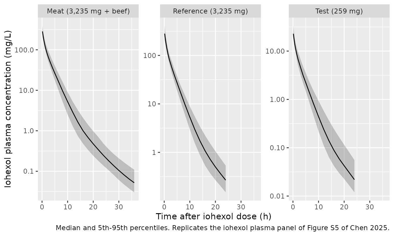

# Replicates the creatinine plasma panel of Figure S5 and the meat-period rise
# of Figure S6 of Chen 2025.
sim |>
  group_by(period, time) |>
  summarise(Q05 = quantile(Cc_creatinine, 0.05), Q50 = median(Cc_creatinine),
            Q95 = quantile(Cc_creatinine, 0.95), .groups = "drop") |>
  ggplot(aes(time, Q50)) +
  geom_ribbon(aes(ymin = Q05, ymax = Q95), alpha = 0.25) +
  geom_line() +
  facet_wrap(~period) +
  labs(x = "Time after iohexol dose (h)", y = "Creatinine plasma concentration (mg/L)",
       caption = "Median and 5th-95th percentiles. Creatinine is flat in the fasting periods and rises after the beef meal (Figures S5, S6 of Chen 2025).")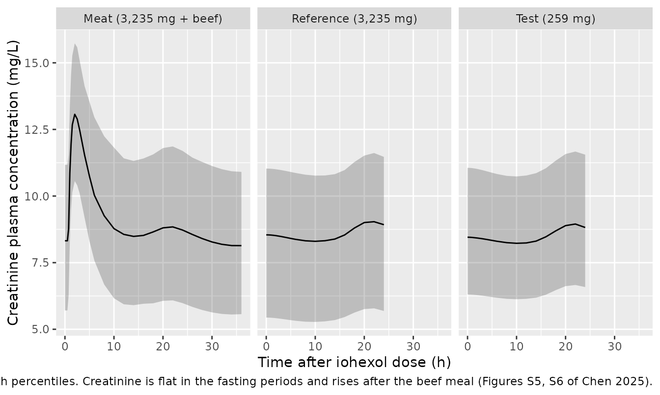

The fasting periods are flat because creatinine sits at its endogenous steady state; only the meat period shows the absorption peak that makes creatinine Vd identifiable. That contrast is the paper’s central study-design argument.

PKNCA validation

Chen 2025 computed clearance in exactly one way (supplement, “Non-compartmental analysis”): the amount excreted in urine over a collection interval divided by the plasma AUC over the same interval, then averaged across intervals within a period. The block below reproduces that method with PKNCA, using the study’s own urine collection windows, so the simulated numbers are scored on the same quantity the answer key reports.

# Descriptive single-dose iohexol NCA. Only `!is.na(Cc)` is filtered so the
# time-zero record that anchors AUC is retained.
nca_in <- sim |>
  filter(!is.na(Cc)) |>
  select(id, time, Cc, period)

conc_iox <- PKNCA::PKNCAconc(as.data.frame(nca_in), Cc ~ time | period + id,
                             concu = "mg/L", timeu = "h")
dose_iox <- PKNCA::PKNCAdose(
  as.data.frame(events |> filter(evid == 1L, cmt == "central") |>
                  select(id, time, amt, period)),
  amt ~ time | period + id, doseu = "mg"
)
iv_single <- data.frame(start = 0, end = Inf, cmax = TRUE, tmax = TRUE,
                        aucinf.obs = TRUE, half.life = TRUE, cl.obs = TRUE)
nca_iox <- suppressWarnings(
  PKNCA::pk.nca(PKNCA::PKNCAdata(conc_iox, dose_iox, intervals = iv_single))
)

as.data.frame(nca_iox$result) |>
  filter(PPTESTCD %in% c("cmax", "tmax", "aucinf.obs", "half.life")) |>
  group_by(period, PPTESTCD) |>
  summarise(Median = median(PPORRES, na.rm = TRUE), .groups = "drop") |>
  tidyr::pivot_wider(names_from = PPTESTCD, values_from = Median) |>
  rename("Period" = period, "Cmax (mg/L)" = cmax, "Tmax (h)" = tmax,
         "AUCinf (mg*h/L)" = aucinf.obs, "Terminal half-life (h)" = half.life) |>
  knitr::kable(digits = 2, caption = "Descriptive iohexol NCA by study period (medians). Chen 2025 does not tabulate these; they are reported for orientation.")

Descriptive iohexol NCA by study period (medians). Chen 2025 does not tabulate these; they are reported for orientation.
Period	AUCinf (mg*h/L)	Cmax (mg/L)	Terminal half-life (h)
Meat (3,235 mg + beef)	552.74	345.34	6.13
Reference (3,235 mg)	565.39	337.79	4.25
Test (259 mg)	46.45	27.76	4.35

Because iohexol is given intravenously and is assumed to be eliminated solely renally, Dose / AUCinf must equal the model’s own clearance. This is a per-subject identity, so it is checked per subject rather than on the group medians.

cl_model <- sim |>
  filter(period == "Test (259 mg)") |>
  group_by(id) |>
  # cir varies over the day, so the identity holds against the DAY-AVERAGED
  # clearance rather than the value at any single time.
  summarise(cl_mean = mean(cl[time <= 24]), .groups = "drop")

cl_nca <- as.data.frame(nca_iox$result) |>
  filter(PPTESTCD == "cl.obs", period == "Test (259 mg)") |>
  select(id, cl_nca = PPORRES)

ident <- inner_join(cl_model, cl_nca, by = "id") |>
  mutate(pct_diff = 100 * (cl_nca - cl_mean) / cl_mean)

sprintf("Dose/AUCinf vs day-averaged model CL: median %+.2f%%, 95%% of subjects within %.2f%%",
        median(ident$pct_diff), max(abs(quantile(ident$pct_diff, c(0.025, 0.975)))))
#> [1] "Dose/AUCinf vs day-averaged model CL: median +1.23%, 95% of subjects within 1.54%"
stopifnot(abs(median(ident$pct_diff)) < 5)

Renal clearance per urine collection interval

# Urine collection windows (Methods, "Study design"): 0-2, 2-4, ..., 20-24 h in
# every period, extended to 36 h in the meat period.
windows <- tibble::tibble(
  start = c(0, 2, 4, 6, 8, 10, 12, 16, 20, 24, 28, 32),
  end   = c(2, 4, 6, 8, 10, 12, 16, 20, 24, 28, 32, 36)
)

interval_clr <- function(conc_col, urine_col, analyte) {
  d <- sim |>
    filter(!is.na(.data[[conc_col]])) |>
    transmute(id, time, Cc = .data[[conc_col]], period)
  iv <- windows |> filter(end <= max(d$time)) |> mutate(auclast = TRUE) |> as.data.frame()
  cobj <- PKNCA::PKNCAconc(as.data.frame(d), Cc ~ time | period + id,
                           concu = "mg/L", timeu = "h")
  res <- suppressWarnings(suppressMessages(
    PKNCA::pk.nca(PKNCA::PKNCAdata(cobj, intervals = iv))
  ))
  auc <- as.data.frame(res$result) |>
    filter(PPTESTCD == "auclast") |>
    transmute(period, id, start, end, auc = PPORRES)
  ae <- sim |>
    group_by(period, id) |>
    reframe(start = iv$start, end = iv$end,
            ae = approx(time, .data[[urine_col]], iv$end)$y -
                 approx(time, .data[[urine_col]], iv$start)$y)
  inner_join(auc, ae, by = c("period", "id", "start", "end")) |>
    mutate(analyte = analyte, clr = ae / auc * 1000 / 60)   # L/h -> mL/min
}

clr <- bind_rows(
  interval_clr("Cc", "Aurine", "Iohexol"),
  interval_clr("Cc_creatinine", "Aurine_creatinine", "Creatinine")
) |>
  filter(!is.na(clr))

# One value per subject per period, as Chen 2025 did before averaging.
clr_subject <- clr |>
  group_by(analyte, period, id) |>
  summarise(clr = mean(clr), .groups = "drop")

# Replicates Figure S7 of Chen 2025: individual iohexol and creatinine
# clearances by urine collection interval, both showing a diurnal pattern with
# higher values during the day and lower values at night.
clr |>
  mutate(mid = (start + end) / 2) |>
  group_by(analyte, mid) |>
  summarise(Q25 = quantile(clr, 0.25), Q50 = median(clr), Q75 = quantile(clr, 0.75),
            .groups = "drop") |>
  ggplot(aes(mid, Q50, colour = analyte, fill = analyte)) +
  geom_ribbon(aes(ymin = Q25, ymax = Q75), alpha = 0.2, colour = NA) +
  geom_line() + geom_point() +
  annotate("rect", xmin = 14, xmax = 24, ymin = -Inf, ymax = Inf, alpha = 0.06) +
  labs(x = "Midpoint of urine collection interval (h)",
       y = "Renal clearance (mL/min)", colour = NULL, fill = NULL,
       caption = "Shaded band = the model's 14-24 h night window. Replicates Figure S7 of Chen 2025.")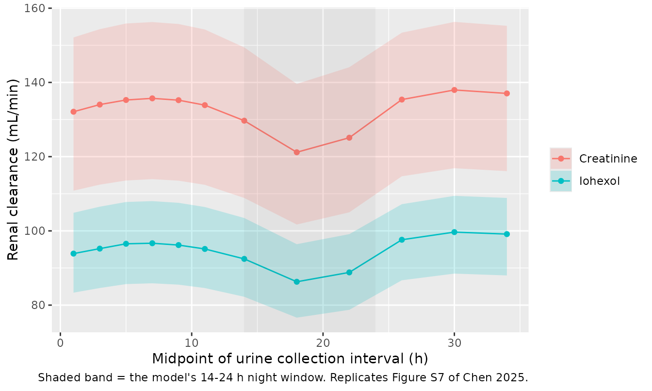

The simulated clearances peak in the middle of the daytime window and trough in the middle of the night window, matching the supplement’s description of Figure S7 (“both exhibiting similar diurnal patterns, with higher values during the day and lower at night”).

Comparison against published NCA

Table S3 of Chen 2025 reports mean (SD) iohexol and creatinine clearance by study period, computed by the interval method above. The comparison uses means, matching the paper’s own aggregation.

simulated <- clr_subject |>
  group_by(analyte, period) |>
  summarise(clr.obs = mean(clr), .groups = "drop") |>
  rename(Analyte = analyte, Period = period)

# Chen 2025 supplement, Table S3, "Iohexol clearance" and "Creatinine
# clearance" columns (mL/min), mean over subjects.
published <- tibble::tribble(
  ~Analyte,     ~Period,                    ~clr.obs,
  "Iohexol",    "Reference (3,235 mg)",      87.2,
  "Iohexol",    "Test (259 mg)",             98.2,
  "Iohexol",    "Meat (3,235 mg + beef)",    98.7,
  "Creatinine", "Reference (3,235 mg)",     127,
  "Creatinine", "Test (259 mg)",            134,
  "Creatinine", "Meat (3,235 mg + beef)",   139
)

cmp <- nlmixr2lib::ncaComparisonTable(
  simulated     = simulated,
  reference     = published,
  by            = c("Analyte", "Period"),
  units         = c(clr.obs = "mL/min"),
  tolerance_pct = 20
)
stopifnot(nrow(cmp) == 6L)   # every reference row must have found a simulated partner

knitr::kable(cmp, align = c("l", "l", "l", "r", "r", "r"),
             caption = "Simulated vs. published renal clearance (Chen 2025 Table S3). * differs from reference by more than 20%.")

Simulated vs. published renal clearance (Chen 2025 Table S3). * differs from reference by more than 20%.
NCA parameter	Analyte	Period	Reference	Simulated	% diff
CLr (obs) (mL/min)	Iohexol	Reference (3,235 mg)	87.2	94.3	+8.1%
CLr (obs) (mL/min)	Iohexol	Test (259 mg)	98.2	93.3	-5.0%
CLr (obs) (mL/min)	Iohexol	Meat (3,235 mg + beef)	98.7	96.4	-2.3%
CLr (obs) (mL/min)	Creatinine	Reference (3,235 mg)	127	132	+3.8%
CLr (obs) (mL/min)	Creatinine	Test (259 mg)	134	130	-2.8%
CLr (obs) (mL/min)	Creatinine	Meat (3,235 mg + beef)	139	134	-3.9%

No row differs from the published value by more than 20%.

# Chen 2025 Table S3, "All" row (n = 14), joined BY ANALYTE rather than by row
# position so a change in grouping order cannot transpose the reference values.
published_all <- tibble::tibble(
  analyte      = c("Iohexol", "Creatinine"),
  Published    = c(95.1, 133),
  `Published SD` = c(21.0, 32)
)

pooled <- clr_subject |>
  group_by(analyte) |>
  summarise(Simulated = mean(clr), `Simulated SD` = sd(clr), .groups = "drop") |>
  inner_join(published_all, by = "analyte") |>
  mutate(`% diff` = 100 * (Simulated - Published) / Published)

stopifnot(nrow(pooled) == 2L)   # a lookup that matched nothing must not pass silently

knitr::kable(pooled, digits = 1,
             caption = "All periods pooled, against the 'All' row of Chen 2025 Table S3 (n = 14).")

All periods pooled, against the ‘All’ row of Chen 2025 Table S3 (n = 14).
analyte	Simulated	Simulated SD	Published	Published SD	% diff
Creatinine	131.9	26.5	133.0	32	-0.8
Iohexol	94.7	15.4	95.1	21	-0.5


stopifnot(all(abs(pooled$`% diff`) < 5))

sd_iohexol <- pooled$`Simulated SD`[pooled$analyte == "Iohexol"]
max_pct_diff <- max(abs(pooled$`% diff`))

Pooled across periods the model lands within 0.8% of the observed means for both analytes. Per period, the reference-period iohexol clearance is the one row that differs materially: Chen 2025 measured 87.2 mL/min there against 98.2 mL/min in the test period, i.e. an apparent iohexol dose effect between the 3,235 mg and 259 mg doses. The joint model contains no dose effect on clearance, so it predicts the same value for all three periods. This is a known and deliberate gap, not a transcription error - the Methods state that the two dose levels were included “to assess a possible dose effect on iohexol clearance; however, it is not the primary objective of this study and will be reported separately.”

The simulated standard deviations are smaller than the observed ones (15 vs 21.0 mL/min for iohexol) because the simulation carries only between-subject variability: residual error, urine-collection error and the between-period dose effect all contribute to the observed spread.

Creatinine Vd and the diagnosis of acute kidney injury

The paper’s main clinical argument is that a wrong creatinine Vd biases how quickly a fall in GFR is detected from plasma creatinine. Chen 2025 simulated a 75% reduction in both GFR and nCTS and read off the times to reach the RIFLE thresholds of 1.5-fold (risk), 2.0-fold (injury) and 3.0-fold (failure) of baseline, under Vd settings of 41.3% (this model), 60.0% and 73.8% of total body weight. Circadian rhythm is switched off for this simulation, as in the paper.

The packaged model starts creatinine at its own steady state, which after the clearance reduction would be the post-AKI plateau rather than the pre-AKI baseline. One line is therefore replaced so the baseline can be supplied as data; everything else about the model is untouched.

mod_aki <- rxode2::model(mod_typ, central_creatinine(0) <- CBASE * vc_creatinine)
#> ℹ add covariate `CBASE`

wt_ref <- 78.5; age_ref <- 33; sexf_ref <- 0
base_row <- data.frame(id = 1L, time = 0, evid = 0L, amt = NA_real_, cmt = "central",
                       dvid = 1L, WT = wt_ref, AGE = age_ref, SEXF = sexf_ref)
base <- rxode2::rxSolve(mod_typ, base_row, useLinCmt = FALSE, returnType = "data.frame")
#> ℹ omega/sigma items treated as zero: 'etalcl', 'etalvc', 'etalvp', 'etalvp2', 'etalcl_tsnet_creatinine', 'etalvc_creatinine', 'etalksyn_creatinine', 'etalfdepot_creatinine'
cbase <- base$Cc_creatinine[1]

aki_times <- seq(0, 96, by = 0.02)
run_aki <- function(vd_pct) {
  ev <- data.frame(id = 1L, time = aki_times, evid = 0L, amt = NA_real_, cmt = "central",
                   dvid = 1L, WT = wt_ref, AGE = age_ref, SEXF = sexf_ref, CBASE = cbase)
  rxode2::rxSolve(
    mod_aki, ev,
    params = c(
      lcl                  = log(5.22317 * 0.25),   # 75% reduction in GFR
      lcl_tsnet_creatinine = log(2.38177 * 0.25),   # 75% reduction in nCTS
      lvc_creatinine       = log(vd_pct / 100 * 70),# Vd as a % of TBW, at the 70 kg reference
      cl_circ_famp_day     = 0,                     # circadian excluded, as in the paper
      cl_circ_famp_night   = 0
    ),
    useLinCmt = FALSE, returnType = "data.frame"
  ) |>
    transmute(time, vd_pct = vd_pct, ratio = Cc_creatinine / cbase)
}
aki <- bind_rows(lapply(c(41.3, 60.0, 73.8), run_aki))
#> ℹ omega/sigma items treated as zero: 'etalcl', 'etalvc', 'etalvp', 'etalvp2', 'etalcl_tsnet_creatinine', 'etalvc_creatinine', 'etalksyn_creatinine', 'etalfdepot_creatinine'
#> ℹ omega/sigma items treated as zero: 'etalcl', 'etalvc', 'etalvp', 'etalvp2', 'etalcl_tsnet_creatinine', 'etalvc_creatinine', 'etalksyn_creatinine', 'etalfdepot_creatinine'
#> ℹ omega/sigma items treated as zero: 'etalcl', 'etalvc', 'etalvp', 'etalvp2', 'etalcl_tsnet_creatinine', 'etalvc_creatinine', 'etalksyn_creatinine', 'etalfdepot_creatinine'

# Replicates Figure 2b of Chen 2025: creatinine concentration-time curves after
# a 75% reduction in GFR and nCTS, under three creatinine Vd assumptions.
ggplot(aki, aes(time, ratio * cbase / 10, colour = factor(vd_pct))) +
  geom_line() +
  geom_hline(yintercept = cbase / 10 * c(1.5, 2, 3), linetype = "dashed", linewidth = 0.3) +
  annotate("text", x = 95, y = cbase / 10 * c(1.5, 2, 3), vjust = -0.4, hjust = 1, size = 3,
           label = c("RIFLE risk (1.5x)", "RIFLE injury (2.0x)", "RIFLE failure (3.0x)")) +
  labs(x = "Time after onset of AKI (h)", y = "Plasma creatinine (mg/dL)",
       colour = "Creatinine Vd\n(% of body weight)",
       caption = "Replicates Figure 2b of Chen 2025.")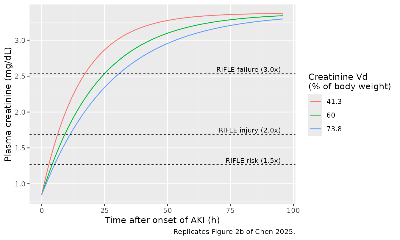

threshold_time <- function(d, k) {
  if (max(d$ratio) < k) return(NA_real_)
  approx(d$ratio, d$time, k, ties = "ordered")$y
}
rifle <- aki |>
  group_by(vd_pct) |>
  group_modify(~ tibble::tibble(risk    = threshold_time(.x, 1.5),
                                injury  = threshold_time(.x, 2.0),
                                failure = threshold_time(.x, 3.0))) |>
  ungroup() |>
  mutate(vd_L = vd_pct / 100 * wt_ref)

rifle |>
  select(vd_pct, vd_L, risk, injury, failure) |>
  rename("Creatinine Vd (% of body weight)" = vd_pct, "Creatinine Vd (L)" = vd_L,
         "Time to RIFLE risk (h)" = risk, "Time to RIFLE injury (h)" = injury,
         "Time to RIFLE failure (h)" = failure) |>
  knitr::kable(digits = 1, caption = "Simulated time from AKI onset to each RIFLE threshold, by assumed creatinine Vd.")

Simulated time from AKI onset to each RIFLE threshold, by assumed creatinine Vd.
Creatinine Vd (% of body weight)	Creatinine Vd (L)	Time to RIFLE risk (h)	Time to RIFLE injury (h)	Time to RIFLE failure (h)
41.3	32.4	2.9	6.3	17.2
60.0	47.1	4.1	9.2	25.0
73.8	57.9	5.1	11.3	30.7


# Select by Vd value rather than by row position.
at_vd <- function(col, vd) {
  v <- rifle[[col]][rifle$vd_pct == vd]
  if (length(v) != 1L || is.na(v)) stop("no unique ", col, " time at Vd = ", vd, "%")
  v
}
time_ratio <- function(col) at_vd(col, 73.8) / at_vd(col, 41.3)

ratios <- tibble::tibble(
  Quantity  = c("Vd ratio (73.8% / 41.3%)", "Time-to-risk ratio", "Time-to-injury ratio",
                "Time-to-failure ratio"),
  Simulated = c(73.8 / 41.3, time_ratio("risk"), time_ratio("injury"), time_ratio("failure"))
)
knitr::kable(ratios, digits = 3, caption = "Chen 2025 Results: 'the ratio of the times is approximately equal to the ratio of Vd used'.")

Chen 2025 Results: ‘the ratio of the times is approximately equal to the ratio of Vd used’.
Quantity	Simulated
Vd ratio (73.8% / 41.3%)	1.787
Time-to-risk ratio	1.787
Time-to-injury ratio	1.787
Time-to-failure ratio	1.787


# The published claim: threshold times scale in proportion to the assumed Vd.
stopifnot(
  abs(time_ratio("risk")    - 73.8 / 41.3) < 0.01,
  abs(time_ratio("injury")  - 73.8 / 41.3) < 0.01,
  abs(time_ratio("failure") - 73.8 / 41.3) < 0.01
)

The model reproduces the paper’s stated proportionality exactly, because with a constant generation rate and first-order elimination the whole post-AKI trajectory depends on time only through CL * t / Vd, so scaling Vd scales every threshold time by the same factor. The paper’s absolute times (4.1-6.5 h to RIFLE risk, 19.6-34.0 h to RIFLE failure) are longer than the simulated ones (2.9-5.1 h and 17.2-30.7 h); see the Errata below for why.

The same curves show the mechanism behind the paper’s other AKI finding - that a pair of samples at 24 h and 48 h gives “minor differences in prediction accuracy” across Vd settings, whereas samples in the first hours do not. After a fractional reduction f in clearance the new plateau is CGR / (f * CL), i.e. 1 / f times baseline, an expression with no Vd term in it at all. Vd sets only how fast each curve travels to that shared plateau.

# The post-AKI plateau is CGR / (0.25 * CL) = 4 x baseline for every Vd: the
# reduction factor cancels CGR and CL, and Vd does not enter a steady state.
plateau <- 1 / 0.25
stopifnot(abs(max(aki$ratio) - plateau) / plateau < 0.01)   # curves do reach it

aki |>
  filter(time %in% c(1, 2, 3, 6, 12, 24, 48, 72)) |>
  mutate(pct = 100 * ratio / plateau) |>
  select(time, vd_pct, pct) |>
  tidyr::pivot_wider(names_from = vd_pct, values_from = pct,
                     names_prefix = "Vd = ", names_glue = "Vd = {vd_pct}% of body weight") |>
  rename("Time after AKI onset (h)" = time) |>
  knitr::kable(digits = 1, caption = "Percentage of the shared, Vd-free post-AKI plateau reached by each Vd assumption.")

Percentage of the shared, Vd-free post-AKI plateau reached by each Vd assumption.
Time after AKI onset (h)	Vd = 41.3% of body weight	Vd = 60% of body weight	Vd = 73.8% of body weight
1	29.6	28.2	27.6
2	34.0	31.3	30.2
3	38.1	34.3	32.6
6	48.9	42.4	39.5
12	65.2	55.8	51.2
24	83.8	73.9	68.2
48	96.5	90.9	86.5
72	99.2	96.8	94.3

At 24 h the three assumptions still span 68-84% of the plateau, so a concentration measured there is genuinely Vd-dependent; by 72 h all three are within 94-99% of the same value, and a 24 h / 48 h pair brackets that approach well enough to pin the reduced clearance without needing Vd to be right. This reproduces the paper’s mechanism, not its reported error percentages: quantifying how badly a mis-specified Vd biases an estimated GFR requires re-fitting the simulated data, which is estimation rather than simulation and is outside this vignette’s scope (see the Errata).

Assumptions and deviations

Sources used. The main article and its Supporting Information (CPT-118-510-s001.docx) were both used. The supplement contains the complete deposited NONMEM control stream, which is the authoritative source for every value in the model file; Table 3 of the article was used as a cross-check. All values are from the paper or its supplement; nothing was digitised from a figure and no value came from correspondence.

Three IIV variances in Table 3 are wrong; the control stream is used. Table 3 reports each IIV as an estimated variance and, separately, as a CV(%). For five of the eight parameters the two agree under CV = sqrt(exp(omega^2) - 1). For three they do not, and in every case the CV(%) column back-transforms exactly to the deposited $OMEGA value while the Estimate column does not:

Parameter	Table 3 Estimate	Table 3 CV(%)	Control stream `$OMEGA`	CV(%) implied by `$OMEGA`
GFR	0.0226	11.9	0.0140315	11.9
Creatinine Vd	0.0211	15.1	0.0226214	15.1
F1	0.00810	10.4	0.0107643	10.4

Two independent lines of evidence confirm the control stream. First, the Results narrative reports that IIV on GFR, iohexol Vc, nCTS and creatinine Vd fell to “11.8%, 14.5%, 32.3% and 15.4%” once allometry was added; Table 3’s final CV column (11.9, 14.6, 23.1, 15.1) continues that trend, whereas an Estimate of 0.0226 on GFR implies 15.1% - higher than the 14.6% reported before any covariate was added. Second, the printed GFR Estimate of 0.0226 sits almost exactly on the upper bound of its own bootstrap confidence interval (0.00379, 0.0246), which a point estimate should not. The pattern looks like a copy error in the Estimate column: the value printed for GFR is creatinine Vd’s, and the value printed for creatinine Vd is an exact duplicate of iohexol Vc’s.

The SEX column polarity in Table 3’s footnote contradicts the model code. Table 3 footnote a states “SEX is a categorical covariate of 0 for male and 1 for female”, but the control stream codes both sex effects as theta^(1 - SEX) - (0.85**(1-SEX)) inside the Cockcroft-Gault term and THETA(15)**(1-SEX) on nCTS. Since Cockcroft-Gault applies its 0.85 factor to women, the dataset column must have been 1 for male and 0 for female, the opposite of the footnote. Table 2’s demographics settle it independently: the tabulated creatinine generation rate is 78.4 mg/h for men, which is (140 - 31) * 86.2 / 72 * 0.6 with no 0.85 factor, and 48.0 mg/h for women, which is (140 - 37) * 64.5 / 72 * 0.6 * 0.85 = 47.1. The model file uses the canonical SEXF column (1 = female) with 0.85^SEXF and 0.628^SEXF, which reproduces both tabulated values and leaves nCTS in women at 62.8% of the male value, consistent with the Discussion’s “higher abundance and expression of transporters in males”.

Allometric exponent of 1 is applied to all four volumes. Table 3’s covariate row is labelled “TBW on iohexol Vc and creatinine Vd”, omitting Vp1 and Vp2, but the Methods are explicit that the exponent of 1.0 applies “for iohexol central compartment volume (Vc), creatinine Vd, and iohexol peripheral compartment volumes (Vp1 and Vp2)”, the Results say TBW was included “as a covariate for all parameters by standard allometric scaling”, and the control stream applies TBWonV to V_CRE, V1_IOX, V2_IOX and V3_IOX alike. The row label is treated as incomplete.

The circadian rhythm is made 24 h periodic. The deposited $PK block implements the rhythm with a DAY = 1 / DAY = 2 latch keyed on TIME .LT. 24, and its night branch fires only for 14 <= TIME <= 24. Over the study’s 0-36 h horizon this is exactly a 24 h periodic function; beyond about 38 h the day branch runs on into negative sine values instead of repeating the night phase, which is an artefact of a latch written for a 36 h study rather than a modelling choice. The model file therefore computes time of day as t - 24 * floor(t / 24), which is numerically identical to the control stream everywhere the model was fit and generalises correctly to longer simulations. Table 3 prints both amplitudes as positive percentages; the nocturnal minus sign comes from the control stream and is confirmed by the Results statement that GFR and nCTS “fluctuated between 104% and 91.6% of the mean over 24 hours”.

A typographical defect in the deposited $DES. The $PK block defines K7 = Q2_IOX/V3_IOX while $DES uses K71 in both the central and the second-peripheral equations. The intended name is K71, matching the K16 / K61 pair used for the first peripheral compartment: with the return rate genuinely absent, the second peripheral compartment would be a one-way sink and neither Qp2 nor Vp2 would be identifiable, yet both are estimated with 8.0% and 3.1% relative standard error. The model file implements the standard two-way peripheral compartment.

Iohexol dose in Table S3. The article’s Methods give the high iohexol dose as 3,235 mg in both the pilot and main study descriptions; footnote a of Table S3 gives it as 3,259 mg. The vignette uses 3,235 mg. Iohexol clearance is linear in this model, so the choice does not affect any clearance comparison.

No iohexol dose effect on clearance. Table S3 shows measured iohexol clearance of 87.2 mL/min in the 3,235 mg reference period against 98.2 mL/min in the 259 mg test period. The joint model has no dose effect, so it predicts one value for all three periods and cannot reproduce this difference. The paper states the dose effect is outside its scope and will be reported separately.

Absolute RIFLE times differ from Figure 2b. The simulated times to the RIFLE thresholds are shorter than the 4.1-6.5 h (risk) and 19.6-34.0 h (failure) the Results report. The simulation above is a forward simulation that changes only Vd while holding clearance at its true reduced value, which makes the threshold times scale exactly with Vd. The paper’s Methods instead describe re-analysing the simulated data with the different Vd settings, which yields a biased clearance estimate as well (the paper reports GFR underestimated by 35.7% and 65.7% at Vd of 60.0% and 73.8%), and a biased clearance shifts the threshold times further. That also explains why the paper’s own ratios (1.59 and 1.74) are only “approximately” the Vd ratio of 1.79, whereas a pure forward simulation reproduces it exactly. Reproducing the re-analysis would require re-estimation rather than simulation and is out of scope for this vignette.

RIFLE thresholds are read against a fixed pre-AKI baseline. The paper does not state which individual supplied Figure 2b beyond “an individual with median dataset covariates”; the vignette uses a male at the cohort mean weight (78.5 kg) and mean age (33 years). Because the threshold times depend on Vd, clearance and the baseline only through the ratio CL * t / Vd, the choice of individual shifts all three thresholds by a common factor and does not affect the proportionality result.

Between-occasion variability is not encoded. IOV on creatinine clearance (3.1%) and on the creatinine generation rate (3.3%) was estimated during model development but “was not included in the final model due to a lack of clinical significance”, so it is absent here.

Parameters without IIV. The deposited $OMEGA fixes the variances on Ka, lag time, Qp1 and Qp2 to zero, so those parameters carry no eta. This matches Table 3, which lists IIV for only eight parameters.

Screened but unused covariates. Height, body mass index, lean body mass, plasma albumin and estimated total body water were tested and not retained. They are recorded in the model file’s covariatesDataExcluded metadata rather than covariateData, so they document the paper’s covariate screen without implying the model needs those columns.

Virtual cohort assumptions. Individual demographics are not published, so weight and age are drawn from sex-specific normal distributions matched to the male and female means and standard deviations of Table 2 and truncated to the observed ranges; sex is drawn with the observed 5-in-14 female fraction. The cohort is 100 subjects per arm rather than the study’s 12-14, so the simulated means are more precise estimates of the model’s central tendency than the published means are of the observed one.

Meat-period creatinine excretion. The model’s meat-period 24 h creatinine excretion exceeds the fasting periods by 401 mg * 52.3% = 210 mg, whereas Table S3’s observed increment is 335 mg. This gap is the paper’s own subject: it reports the same 335 mg figure as the “individual differences in creatinine excretion over 24 h” dose input in Table 1, and the Discussion attributes the discrepancy to interference from the roughly 2,000 mg of endogenous creatinine produced daily, which makes a ~300 mg external load hard to measure by difference. The final model uses the directly measured beef creatinine content with an estimated bioavailability instead.