Berotralstat (Mathis 2022)
Source:vignettes/articles/Mathis_2022_berotralstat.Rmd
Mathis_2022_berotralstat.RmdModel and source
Berotralstat (BCX7353, Orladeyo) is an oral, once-daily small-molecule inhibitor of plasma kallikrein, approved for prophylaxis of attacks of hereditary angioedema (HAE) in adults and adolescents aged 12 years and older. Mathis 2022 pooled 10,437 plasma concentrations from 771 healthy subjects and HAE patients in 13 phase 1-3 studies and described them with a three-compartment model with first-order absorption, an absorption lag time and linear elimination. Body weight acts on clearance and central volume, and relative bioavailability rises with dose.
mod <- rxode2::rxode(readModelDb("Mathis_2022_berotralstat"))
#> ℹ parameter labels from comments will be replaced by 'label()'- Citation: Mathis A, Sale M, Cornpropst M, Sheridan WP, Ma SC. Population pharmacokinetic modeling and simulations of berotralstat for prophylactic treatment of attacks of hereditary angioedema. Clin Transl Sci. 2022;15(4):1027-1035. doi:10.1111/cts.13233. Fixed-effect estimates from Table 1; model code and random-effect values from Supporting Information Text S2.
- Article: https://doi.org/10.1111/cts.13233
- Supporting Information (EuropePMC, open access): https://europepmc.org/article/PMC/PMC9010267
Table 1 of the paper gives the final fixed effects. Supporting
Information Text S2 is the NONMEM control stream of the final model,
which fixes the structure: ADVAN12, the $PK
covariate equations and a combined additive-plus-proportional
$ERROR block. The random-effect variances are a special
case, described under Assumptions and deviations below.
Population
str(mod$population)
#> List of 15
#>  $ species       : chr "human"
#>  $ n_subjects    : num 771
#>  $ n_studies     : num 13
#>  $ n_observations: num 10437
#>  $ age_range     : chr "12-74 years"
#>  $ age_mean      : chr "38.1 years (SD 13.9); median 37 years (Supporting Information Table S3)"
#>  $ weight_range  : chr "40.1-150 kg"
#>  $ weight_median : chr "75.1 kg (mean 77.7 kg, SD 17.2; Supporting Information Table S3); the model is centered on 75.2 kg"
#>  $ sex_female_pct: num 46.3
#>  $ race_ethnicity: Named num [1:6] 83.3 8.7 4.5 2.7 0.4 0.4
#>   ..- attr(*, "names")= chr [1:6] "White" "Asian" "Black" "Other" ...
#>  $ disease_state : chr "Healthy adults (including 7 with severe renal impairment and 18 with Child-Pugh A-C hepatic impairment) and pat"| __truncated__
#>  $ dose_range    : chr "Oral single doses of 10-900 mg and once-daily repeat doses of 110-450 mg (Methods, Clinical trial subjects); th"| __truncated__
#>  $ formulation   : chr "API-in-capsule (dose expressed as the HCl salt; studies BCX7353-101, -102, -103, -105, -203) and blend-in-capsu"| __truncated__
#>  $ regions       : chr "International; study BCX7353-301 (APeX-J) enrolled Japanese patients and Part 3 of BCX7353-101 enrolled Japanes"| __truncated__
#>  $ notes         : chr "Thirteen phase 1-3 studies pooled (Supporting Information Table S1); demographics in Supporting Information Tab"| __truncated__
The 771 subjects (Results, Data summary; Supporting Information Table S3) were aged 12-74 years (mean 38.1, SD 13.9) and weighed 40.1-150 kg (median 75.1 kg). 53.7 percent were male. 83.3 percent were White, 8.7 percent Asian, 4.5 percent Black or African American and 2.7 percent other races. About half were HAE patients: 400 of 771 came from the four patient studies BCX7353-203, -204, -301 and -302. The rest were healthy subjects, including small renal- and hepatic-impairment cohorts. Only 16 subjects were 17 years old or younger. Doses ranged from single doses of 10-900 mg to once-daily doses of 110-450 mg.
Source trace
| Model element | Value | Source |
|---|---|---|
| Structure: 3 compartments, first-order absorption, lag time, linear elimination | – | Results, Final model; Figure 1; Text S2
$SUBROUTINE ADVAN12
|
lcl CL |
47.3 L/h | Table 1 |
lvc V2 |
1650 L | Table 1 |
lk12 K23 |
0.0812 1/h | Table 1 |
lk21 K32 |
0.0309 1/h | Table 1 |
lk13 K24 |
0.00281 1/h | Table 1 |
lk31 K42 |
0.00136 1/h | Table 1 |
lka Ka |
1.12 1/h | Table 1 |
ltlag ALAG1 |
0.468 h | Table 1 |
e_wt_cl |
0.480 | Table 1; Text S2 TVCL= THETA(1)*CWTKG**THETA(15)
|
e_wt_vc |
1.00 | Table 1; Text S2 TVV2=THETA(2)*CWTKG**THETA(13)
|
| Weight reference | 75.2 kg | Table 1 footnote; Text S2 CWTKG =WTKG/75.2
|
e_dose_f, F1 = (Dose/300)^THETA(11) |
0.497 | Table 1; Equation 1; Text S2
F1=1*(DOSE/CDOSE)**THETA(11), CDOSE = 300
|
etalcl, etalvc, etalka,
etaltlag block |
0.141588 … 0.245715 | Text S2 $OMEGA BLOCK(4) (initial estimates) |
eta_study_lcl |
0.0817099 | Text S2 $OMEGA ETA(5), $LEVEL STDY=(5[1])
(initial estimate) |
addSd |
0.483 ng/mL | Table 1; Text S2 W=SQRT(ADDERR**2+PROPERR**2*IPRE**2),
$SIGMA 1 FIX
|
propSd |
0.286 | Table 1 |
Cc = 1000 * central / vc |
– | Text S2 S2 = V2/1000 (dose mg, concentration
ng/mL) |
Typical-value checks
Terminal half-life
The paper reports a terminal half-life of 566 h from the final model (Results, Final model and model evaluation). That is a property of the typical micro-constants alone, so it is checked from the eigenvalues of the disposition rate matrix.
p <- exp(unlist(mod$theta[c("lcl", "lvc", "lk12", "lk21", "lk13", "lk31")]))
kel <- p[["lcl"]] / p[["lvc"]]
rate_matrix <- matrix(
  c(-(kel + p[["lk12"]] + p[["lk13"]]), p[["lk21"]], p[["lk31"]],
    p[["lk12"]], -p[["lk21"]], 0,
    p[["lk13"]], 0, -p[["lk31"]]),
  nrow = 3, byrow = TRUE
)
half_lives <- sort(log(2) / -eigen(rate_matrix)$values)
half_lives
#> [1]   5.079059  95.645839 569.052666

# Deterministic: depends only on the printed Table 1 values. The residual
# 0.5 percent is the rounding of K24 and K42 to three significant figures.
stopifnot(abs(half_lives[3] / 566 - 1) < 0.01)
The three phases have half-lives of about 5 h, 96 h and 569 h. The middle one matches the 93-h NCA half-life of the single-dose studies. The paper’s Discussion explains why: those studies were too short to see the third phase.
Steady-state AUC against its closed form
At steady state the dosing-interval AUC of a linear model is F x Dose / CL. This checks the solve, the bioavailability term and the mg-to-ng/mL scaling together.
typ <- rxode2::zeroRe(mod)
obs_times <- seq(0, 24, by = 0.25)

make_events <- function(wt, dose = 150, ss = 0) {
  rbind(
    data.frame(time = 0, evid = 1L, amt = dose, cmt = "depot",
               ss = ss, ii = if (ss == 1) 24 else 0),
    data.frame(time = obs_times, evid = 0L, amt = 0, cmt = "central",
               ss = 0, ii = 0)
  ) |>
    dplyr::mutate(WT = wt, DOSE_BEROTRALSTAT_MG = dose)
}

trap_auc <- function(time, conc) {
  sum(diff(time) * (head(conc, -1) + tail(conc, -1)) / 2)
}

ss_typ <- rxode2::rxSolve(typ, make_events(75.2, ss = 1), returnType = "data.frame")
#> ℹ omega/sigma items treated as zero: 'etaltlag', 'etalka', 'etalvc', 'etalcl', 'eta_study_lcl'
auc_ss_solve <- trap_auc(ss_typ$time, ss_typ$Cc)
auc_ss_closed <- 1000 * (150 / 300)^0.497 * 150 / 47.3
c(solve = auc_ss_solve, closed_form = auc_ss_closed)
#>       solve closed_form
#>    2246.957    2247.078

# Same drawn (typical) parameters on both sides: the gap is trapezoidal error on
# a 0.25 h grid, so the bound is tight.
stopifnot(abs(auc_ss_solve / auc_ss_closed - 1) < 0.005)
Virtual cohort
Table 2 of the paper simulates 1000 HAE patients per scenario at the commercial dose of 150 mg once daily. Its adult scenarios are four weight bands, with weights drawn from a log-normal distribution whose mean and variance come from the analysis dataset. Here each band gets 200 subjects. Weights are drawn from a log-normal with the Table S3 all-subject mean 77.7 kg and SD 17.2 kg, truncated to the band.
The model has no age effect, so the paper’s adolescent scenario differs from the adults only in its weight distribution. That scenario uses CDC weight-for-age charts, whose parameters the paper does not print, so it is not re-simulated. The adolescent row is checked separately below through the weight it implies.
n_per_band <- 200
bands <- tibble::tribble(
  ~band,                               ~lo, ~hi,
  "Underweight adults (40-60 kg)",      40,  60,
  "Low weight adults (60-80 kg)",       60,  80,
  "Normal weight adults (80-100 kg)",   80, 100,
  "Overweight adults (100-120 kg)",    100, 120
)

sdlog <- sqrt(log(1 + (17.2 / 77.7)^2))
meanlog <- log(77.7) - sdlog^2 / 2

rxode2::rxSetSeed(20220401)
cohort <- bands |>
  dplyr::rowwise() |>
  dplyr::reframe(
    band = band,
    WT = stats::qlnorm(
      stats::runif(n_per_band,
                   stats::plnorm(lo, meanlog, sdlog),
                   stats::plnorm(hi, meanlog, sdlog)),
      meanlog, sdlog
    )
  ) |>
  dplyr::mutate(id = dplyr::row_number())

cohort |>
  dplyr::group_by(band = factor(band, levels = bands$band)) |>
  dplyr::summarise(n = dplyr::n(), median_wt = stats::median(WT),
                   min_wt = min(WT), max_wt = max(WT), .groups = "drop") |>
  dplyr::rename("Weight band" = band, "N" = n, "Median weight (kg)" = median_wt,
                "Min (kg)" = min_wt, "Max (kg)" = max_wt) |>
knitr::kable(digits = 1)| Weight band | N | Median weight (kg) | Min (kg) | Max (kg) |
|---|---|---|---|---|
| Underweight adults (40-60 kg) | 200 | 55.4 | 40.9 | 60.0 |
| Low weight adults (60-80 kg) | 200 | 71.8 | 60.0 | 79.9 |
| Normal weight adults (80-100 kg) | 200 | 87.7 | 80.1 | 99.9 |
| Overweight adults (100-120 kg) | 200 | 106.7 | 100.2 | 119.2 |
Simulation
Each subject is simulated twice: after the first 150 mg dose, and
over one dosing interval at true steady state (ss = 1). The
steady-state option matters here. With a 569-h terminal half-life, even
several months of daily dosing falls short of steady state.
Table 2’s geometric CVs for AUC at steady state are 36.7-38.6 percent. Within a weight band, the CV of that AUC reflects only CL, through F x Dose / CL. The between-subject variance on CL alone (0.1416, a CV of 39 percent) accounts for it. Adding the between-study variance (0.0817) would push it to about 50 percent. The Table 2 replication therefore sets the between-study eta to zero, which appears to be what the paper’s own simulations did. Concentrations are individual predictions without residual error.
mod_no_study <- mod |> rxode2::ini(eta_study_lcl = fix(0))
#> ℹ fix `eta_study_lcl` to `0.0817099`
#> ℹ change initial estimate of `eta_study_lcl` to `0`

build_events <- function(ss) {
  cohort |>
    dplyr::rowwise() |>
    dplyr::reframe(id = id, band = band, make_events(WT, ss = ss)) |>
    as.data.frame()
}

ev_first <- build_events(ss = 0)
ev_ss <- build_events(ss = 1)

rxode2::rxSetSeed(20220402)
sim_first <- rxode2::rxSolve(mod_no_study, ev_first, keep = "band",
                             returnType = "data.frame") |>
  dplyr::mutate(regimen = "First dose")
#> ℹ omega/sigma items treated as zero: 'eta_study_lcl'
# The steady-state solve iterates to convergence over a 569-h terminal phase.
# With the default step limit a few subjects with extreme absorption etas stop
# with "excess work done" and come back as NA, which PKNCA would then drop
# silently. A larger step limit solves them all; the gate below fails loudly
# if any subject is still missing.
rxode2::rxSetSeed(20220402)
sim_ss <- rxode2::rxSolve(mod_no_study, ev_ss, keep = "band",
                          maxsteps = 500000L, returnType = "data.frame") |>
  dplyr::mutate(regimen = "Steady state")
#> ℹ omega/sigma items treated as zero: 'eta_study_lcl'
sim <- dplyr::bind_rows(sim_first, sim_ss)
stopifnot(!anyNA(sim$Cc), dplyr::n_distinct(sim_ss$id) == nrow(cohort))
Replicates Figure 4
sim |>
  dplyr::group_by(regimen, band, time) |>
  dplyr::summarise(median_cc = stats::median(Cc), .groups = "drop") |>
  ggplot(aes(time, median_cc, colour = factor(band, levels = bands$band))) +
  geom_line() +
  facet_wrap(~regimen, scales = "free_y") +
  labs(x = "Time after dose (h)", y = "Median berotralstat (ng/mL)",
       colour = NULL,
       caption = "Replicates Figure 4 of Mathis 2022 (150 mg once daily).") +
  theme_bw() +
  theme(legend.position = "bottom") +
  guides(colour = guide_legend(ncol = 2))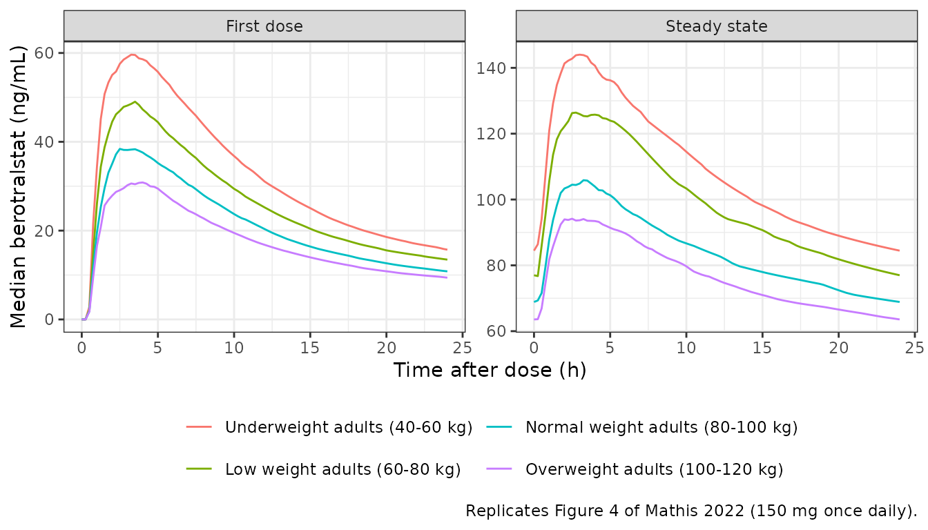
PKNCA validation
run_nca <- function(dat) {
  conc <- dat |>
    dplyr::filter(!is.na(Cc)) |>
    dplyr::select(id, time, Cc, band)
  # One time-zero row per subject. After the first dose it is 0; at steady state
  # it is already in the solve output (the pre-dose trough), and distinct()
  # keeps that row.
  conc <- dplyr::bind_rows(
    conc,
    conc |> dplyr::distinct(id, band) |> dplyr::mutate(time = 0, Cc = 0)
  ) |>
    dplyr::distinct(id, band, time, .keep_all = TRUE) |>
    dplyr::arrange(id, time)
  doses <- conc |> dplyr::distinct(id, band) |> dplyr::mutate(time = 0, amt = 150)
  res <- PKNCA::pk.nca(PKNCA::PKNCAdata(
    PKNCA::PKNCAconc(conc, Cc ~ time | band + id),
    PKNCA::PKNCAdose(doses, amt ~ time | band + id),
    intervals = data.frame(start = 0, end = 24, cmax = TRUE, auclast = TRUE)
  ))
  as.data.frame(res)
}

# One PKNCA call per band and regimen keeps each call to 200 subjects.
nca <- sim |>
  dplyr::group_split(regimen, band) |>
  lapply(function(d) dplyr::mutate(run_nca(d), regimen = d$regimen[1])) |>
  dplyr::bind_rows()

nca_wide <- nca |>
  dplyr::filter(PPTESTCD %in% c("cmax", "auclast")) |>
  dplyr::select(band, id, regimen, PPTESTCD, PPORRES) |>
  tidyr::pivot_wider(names_from = PPTESTCD, values_from = PPORRES)
Comparison against Table 2
gcv <- function(x) 100 * sqrt(exp(stats::var(log(x))) - 1)

published <- tibble::tribble(
  ~band,                              ~auc_first, ~cmax_first, ~auc_ss, ~cmax_ss, ~cv_auc_ss, ~rac,
  "Underweight adults (40-60 kg)",           816,          67,    2574,      155,       36.7, 3.15,
  "Low weight adults (60-80 kg)",            644,          51,    2211,      129,       38.3, 3.43,
  "Normal weight adults (80-100 kg)",        509,          40,    1951,      111,       37.0, 3.83,
  "Overweight adults (100-120 kg)",          438,          34,    1818,      101,       36.9, 4.15
)

simulated <- nca_wide |>
  dplyr::group_by(band) |>
  dplyr::summarise(
    auc_first = exp(mean(log(auclast[regimen == "First dose"]))),
    cmax_first = exp(mean(log(cmax[regimen == "First dose"]))),
    auc_ss = exp(mean(log(auclast[regimen == "Steady state"]))),
    cmax_ss = exp(mean(log(cmax[regimen == "Steady state"]))),
    cv_auc_ss = gcv(auclast[regimen == "Steady state"]),
    .groups = "drop"
  ) |>
  dplyr::mutate(rac = auc_ss / auc_first)

cmp <- dplyr::inner_join(simulated, published, by = "band",
                         suffix = c("_sim", "_pub")) |>
  tidyr::pivot_longer(-band, names_to = c("metric", ".value"),
                      names_pattern = "(.*)_(sim|pub)") |>
  dplyr::mutate(pct_diff = 100 * (sim - pub) / pub)

metric_labels <- c(
  auc_first = "AUC0-24, first dose (ng*h/mL)",
  cmax_first = "Cmax, first dose (ng/mL)",
  auc_ss = "AUCtau, steady state (ng*h/mL)",
  cmax_ss = "Cmax, steady state (ng/mL)",
  cv_auc_ss = "Geometric CV of AUCtau,ss (%)",
  rac = "Accumulation ratio"
)

cmp |>
  dplyr::arrange(match(band, bands$band), match(metric, names(metric_labels))) |>
  dplyr::mutate(metric = metric_labels[metric]) |>
  dplyr::rename("Weight band" = band, "NCA parameter" = metric,
                "Simulated" = sim, "Mathis 2022 Table 2" = pub,
                "% difference" = pct_diff) |>
  knitr::kable(digits = 2, caption = paste(
    "Simulated geometric means (200 subjects per band) against the paper's",
    "Table 2 (1000 per band), 150 mg once daily."
))| Weight band | NCA parameter | Simulated | Mathis 2022 Table 2 | % difference |
|---|---|---|---|---|
| Underweight adults (40-60 kg) | AUC0-24, first dose (ng*h/mL) | 801.87 | 816.00 | -1.73 |
| Underweight adults (40-60 kg) | Cmax, first dose (ng/mL) | 65.32 | 67.00 | -2.51 |
| Underweight adults (40-60 kg) | AUCtau, steady state (ng*h/mL) | 2655.62 | 2574.00 | 3.17 |
| Underweight adults (40-60 kg) | Cmax, steady state (ng/mL) | 149.68 | 155.00 | -3.43 |
| Underweight adults (40-60 kg) | Geometric CV of AUCtau,ss (%) | 37.70 | 36.70 | 2.74 |
| Underweight adults (40-60 kg) | Accumulation ratio | 3.31 | 3.15 | 5.14 |
| Low weight adults (60-80 kg) | AUC0-24, first dose (ng*h/mL) | 648.69 | 644.00 | 0.73 |
| Low weight adults (60-80 kg) | Cmax, first dose (ng/mL) | 51.92 | 51.00 | 1.80 |
| Low weight adults (60-80 kg) | AUCtau, steady state (ng*h/mL) | 2358.18 | 2211.00 | 6.66 |
| Low weight adults (60-80 kg) | Cmax, steady state (ng/mL) | 129.37 | 129.00 | 0.28 |
| Low weight adults (60-80 kg) | Geometric CV of AUCtau,ss (%) | 38.84 | 38.30 | 1.42 |
| Low weight adults (60-80 kg) | Accumulation ratio | 3.64 | 3.43 | 5.99 |
| Normal weight adults (80-100 kg) | AUC0-24, first dose (ng*h/mL) | 519.76 | 509.00 | 2.11 |
| Normal weight adults (80-100 kg) | Cmax, first dose (ng/mL) | 40.70 | 40.00 | 1.74 |
| Normal weight adults (80-100 kg) | AUCtau, steady state (ng*h/mL) | 2017.00 | 1951.00 | 3.38 |
| Normal weight adults (80-100 kg) | Cmax, steady state (ng/mL) | 107.89 | 111.00 | -2.81 |
| Normal weight adults (80-100 kg) | Geometric CV of AUCtau,ss (%) | 40.82 | 37.00 | 10.31 |
| Normal weight adults (80-100 kg) | Accumulation ratio | 3.88 | 3.83 | 1.32 |
| Overweight adults (100-120 kg) | AUC0-24, first dose (ng*h/mL) | 428.92 | 438.00 | -2.07 |
| Overweight adults (100-120 kg) | Cmax, first dose (ng/mL) | 33.58 | 34.00 | -1.23 |
| Overweight adults (100-120 kg) | AUCtau, steady state (ng*h/mL) | 1840.12 | 1818.00 | 1.22 |
| Overweight adults (100-120 kg) | Cmax, steady state (ng/mL) | 96.70 | 101.00 | -4.25 |
| Overweight adults (100-120 kg) | Geometric CV of AUCtau,ss (%) | 34.35 | 36.90 | -6.90 |
| Overweight adults (100-120 kg) | Accumulation ratio | 4.29 | 4.15 | 3.38 |
exposure <- cmp |> dplyr::filter(metric %in% c("auc_first", "cmax_first", "auc_ss", "cmax_ss"))
summary(exposure$pct_diff)
#>    Min. 1st Qu.  Median    Mean 3rd Qu.    Max.
#> -4.2530 -2.1837  0.5063  0.1907  1.8786  6.6569

# Assert on the centre and on a robust quantile, not on the extremes: the
# cohort is a random draw and its tails are not reproducible across rxode2
# builds. A mis-transcribed CL, V2, bioavailability exponent or unit moves the
# whole set by tens of percent.
stopifnot(
  abs(stats::median(exposure$pct_diff)) < 7,
  stats::quantile(abs(exposure$pct_diff), 0.9) < 15
)

# The accumulation ratio is a level-independent ratio of two AUCs from the same
# subjects. It tests the distribution rate constants and the steady-state
# solve, independently of CL and F.
rac <- cmp |> dplyr::filter(metric == "rac")
stopifnot(abs(stats::median(rac$pct_diff)) < 7)

# Variability: the CV of AUCtau,ss is driven by the CL variance. With n = 200
# the sampling error of a CV near 38 percent is about 2 points.
cv <- cmp |> dplyr::filter(metric == "cv_auc_ss")
stopifnot(abs(stats::median(cv$sim - cv$pub)) < 6)
All sixteen geometric means fall within 7 percent of Table 2, with a median difference near zero. The accumulation ratio rises with weight, as in the paper (Table 2: 3.15 to 4.15). The simulated ratios run 1-6 percent above the published ones in every band, because the simulated steady-state AUCs are slightly higher. A likely cause is that the paper’s “steady state” was a long but finite run of daily doses rather than the true steady state used here; with a 569-h terminal phase the two differ by a few percent. The geometric CV of AUC at steady state matches Table 2 within the sampling error of 200 subjects (median gap about 1 point). The control-stream variance on CL, an initial estimate, therefore reproduces the published spread.
Adolescents: the weight Table 2 implies
Within the model, AUC at steady state scales as WT^-0.480 and nothing else differs between adolescents and adults. Inverting the low-weight-adult row gives the typical weight that each Table 2 row implies.
table2_auc_ss <- c(
  "Underweight adults (40-60 kg)" = 2574,
  "Low weight adults (60-80 kg)" = 2211,
  "Normal weight adults (80-100 kg)" = 1951,
  "Overweight adults (100-120 kg)" = 1818,
  "Adolescents (12-18 years)" = 2515
)
implied_wt <- 75.2 * (table2_auc_ss / auc_ss_closed)^(-1 / 0.480)
round(implied_wt, 1)
#>    Underweight adults (40-60 kg)     Low weight adults (60-80 kg)
#>                             56.7                             77.8
#> Normal weight adults (80-100 kg)   Overweight adults (100-120 kg)
#>                            100.9                            116.9
#>        Adolescents (12-18 years)
#>                             59.5
The inversion is sensitive: the exponent 1/0.480 turns a 1 percent AUC difference into a 2 percent weight difference, so the adult rows land near the centre or upper edge of their bands rather than exactly at the typical weight. The adolescent row implies about 60 kg, just above the underweight adults (about 57 kg). This matches the paper’s statement that adolescents and underweight adults have almost equal exposures, and in this model weight is the only covariate that could produce it.
Stochastic VPC with all variability
For completeness, the full model is simulated as shipped: both the between-subject and the between-study random effects, plus residual error. The cohort is 200 subjects at 75.2 kg, after the first 150 mg dose.
vpc_events <- do.call(rbind, lapply(seq_len(200), function(i) {
  dplyr::mutate(make_events(75.2), id = i)
}))
rxode2::rxSetSeed(20220403)
vpc <- rxode2::rxSolve(mod, vpc_events, returnType = "data.frame")

vpc |>
  dplyr::group_by(time) |>
  dplyr::summarise(
    p05 = stats::quantile(sim, 0.05), p50 = stats::median(sim),
    p95 = stats::quantile(sim, 0.95), .groups = "drop"
  ) |>
  ggplot(aes(time, p50)) +
  geom_ribbon(aes(ymin = p05, ymax = p95), alpha = 0.25) +
  geom_line() +
  labs(x = "Time after first 150 mg dose (h)", y = "Berotralstat (ng/mL)",
       caption = "Median and 90% prediction interval, 75.2 kg, full random effects.") +
  theme_bw()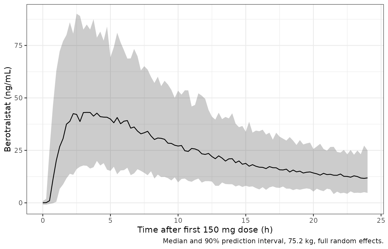
Assumptions and deviations
-
Random-effect variances are control-stream initial
estimates. The paper states which parameters carry
between-subject variability (CL, V2, Ka and the lag time, in one
correlated block) and that a between-study random effect acts on CL. It
does not print the final variances, in Table 1 or in the Supporting
Information. The only values published are the
$OMEGAinitial estimates in the Text S2 final-model control stream, and the model uses those verbatim. They appear to be near-converged: the$THETAinitials in the same file are within 5 percent of the Table 1 finals for every parameter except the poorly determined K24 and K42 (11 and 18 percent; for example CL 47.0 vs 47.3 L/h, V2 1603 vs 1650 L), and the AUC CVs simulated here sit a few points above Table 2. The implied CVs are about 39 percent on CL, 34 percent on V2, 101 percent on Ka and 53 percent on the lag time, plus 29 percent between studies on CL. -
Between-study variability is drawn per subject. In
NONMEM ETA(5) is shared by every subject in a study
(
$LEVEL STDY=(5[1])). In a plainrxSolveit is drawn per subject, which adds to the between-subject spread on CL. Seteta_study_lclto zero to reproduce the paper’s Table 2, as above. To mimic a multi-study trial, draw it once per study and pass it in as a data column. -
Dose covariate.
DOSE_BEROTRALSTAT_MGmust equal the dose amount. In the source, API-in-capsule doses are expressed as the HCl salt and blend-in-capsule (commercial) doses as the free base. The two were bioequivalent at those nominal doses (Table S2). - Figure 1 caption. The caption says “higher doses predicting lower bioavailability”. Equation 1, the positive THETA(11) of 0.497, the Study Highlights and the Discussion all say the opposite: bioavailability rises with dose. The model follows the equation.
- Dose range. The Methods quote single doses of 10-900 mg. Supporting Information Table S1 lists study BCX7353-101 Part 1 doses up to 1000 mg. The population metadata uses the Methods range.
-
BLQ handling and the assay switch. The control
stream fits BLQ records with the M3 likelihood. It also computes an
ASSAYflag that the final$ERRORblock never uses. Neither affects simulation.