Nivolumab in Japanese NSCLC (Tohi 2023)
Source:vignettes/articles/Tohi_2023_nivolumab.Rmd
Tohi_2023_nivolumab.RmdModel and source
- Citation: Tohi M, Irie K, Mizuno T, Okuyoshi H, Hirabatake M, Ikesue H, Muroi N, Eto M, Fukushima S, Tomii K, Hashida T. Population Pharmacokinetics of Nivolumab in Japanese Patients with Nonsmall Cell Lung Cancer. Ther Drug Monit. 2023;45(1):110-116. doi:10.1097/FTD.0000000000000996
- Description: Two-compartment population PK model for intravenous nivolumab (anti-PD-1 IgG4) in Japanese adults with non-small cell lung cancer, with power effects of serum albumin and eGFR on clearance and a sigmoid Emax decrease of clearance with time since the first dose (Tohi 2023)
- Article: https://doi.org/10.1097/FTD.0000000000000996 (open access, PMC9819210)
- Supplemental Digital Content 1: Table S1 (forward covariate inclusion), Table S2 (backward elimination), Table S3 (longitudinal albumin and eGFR) and Figure S1 (Monte Carlo trough concentrations by regimen, albumin and eGFR).
Tohi et al. fitted a population PK model to 223 opportunistically sampled remnant-serum nivolumab concentrations from 34 Japanese patients with non-small cell lung cancer (NSCLC) treated with 240 mg nivolumab monotherapy in routine care. The structural model is two-compartment with first-order elimination. Clearance depends on serum albumin (negative power effect), eGFR (positive power effect), and a sigmoid Emax decrease with time since the first dose whose three parameters were held at the values of Osawa et al. (2019, gastric cancer); the data could not estimate them.
mod <- readModelDb("Tohi_2023_nivolumab")
ui <- rxode2::rxode(mod)
#> ℹ parameter labels from comments will be replaced by 'label()'
ui
#>  ── rxode2-based free-form 2-cmt ODE model ──────────────────────────────────────
#>  ── Initalization: ──
#> Fixed Effects ($theta):
#>           lcl           lvc           lvp            lq      e_alb_cl
#>    -5.0514573     0.8241754     0.5933268    -4.0173835    -1.4800000
#>     e_crcl_cl   cl_time_max       lcl_t50 lcl_time_hill        propSd
#>     0.4110000    -0.2850000     7.3198649     0.7030975     0.1600000
#>
#> Omega ($omega):
#>         etalcl  etalvc
#> etalcl 0.03695 0.00000
#> etalvc 0.00000 0.19425
#> attr(,"lotriLabels")
#> [1] "Table 2: IIV for CL = 19.4 CV%; log(1 + 0.194^2) = 0.03695"
#> [2] "Table 2: IIV for V1 = 46.3 CV%; log(1 + 0.463^2) = 0.19425"
#> attr(,"lotriFix")
#>        etalcl etalvc
#> etalcl  FALSE  FALSE
#> etalvc  FALSE  FALSE
#>
#> States ($state or $stateDf):
#>   Compartment Number Compartment Name
#> 1                  1          central
#> 2                  2      peripheral1
#>  ── μ-referencing ($muRefTable): ──
#>   theta    eta level
#> 1   lcl etalcl    id
#> 2   lvc etalvc    id
#>
#>  ── Model (Normalized Syntax): ──
#> function() {
#>     compartmentData <- list(central = list(analyte = "nivolumab",
#>         units = "mg", specimen = "serum", verified = TRUE), peripheral1 = list(analyte = "nivolumab",
#>         units = "mg", specimen = "serum", verified = TRUE))
#>     covariateData <- list(ALB = list(description = "Serum albumin",
#>         units = "g/L", type = "continuous", reference_category = NULL,
#>         notes = "Time-varying (measured approximately every 2 weeks; Methods 'Covariate Analysis on Nivolumab Clearance'). Power effect on CL with reference 3.6 g/dL (the Table 1 median and the value printed in the final CL equation). The source reports albumin in g/dL; the canonical column is g/L, so model() converts with alb_gdL <- ALB * 0.1 before applying the published coefficient.",
#>         source_name = "ALB"), CRCL = list(description = "Estimated glomerular filtration rate, BSA-normalized",
#>         units = "mL/min/1.73 m^2", type = "continuous", reference_category = NULL,
#>         notes = "Time-varying eGFR calculated with the Japanese-population equation (Methods 'Patients', reference 14 of the source). Power effect on CL with reference 70 mL/min/1.73 m^2 (the Table 1 median and the value printed in the final CL equation).",
#>         source_name = "eGFR"))
#>     covariatesDataExcluded <- list(AGE = list(description = "Age",
#>         units = "years", type = "continuous", reference_category = NULL,
#>         notes = "Screened on CL in the forward-inclusion step (Table S1, dOFV -0.41, p = 0.522) and not retained."),
#>         WT = list(description = "Body weight", units = "kg",
#>             type = "continuous", reference_category = NULL, notes = "Screened on CL as a time-varying covariate (Table S1, dOFV -0.365, p = 0.546) and not retained. Body weight enters only the 3 mg/kg dose in the published Monte Carlo simulation."),
#>         BSA = list(description = "Body surface area", units = "m^2",
#>             type = "continuous", reference_category = NULL, notes = "Screened on CL as a time-varying covariate (Table S1, dOFV -0.944, p = 0.331) and not retained."),
#>         SEXF = list(description = "Biological sex, 1 = female",
#>             units = "(binary)", type = "binary", reference_category = "0 (male)",
#>             notes = "Screened on CL (Table S1, dOFV -0.011, p = 0.916) and not retained."),
#>         ECOG = list(description = "ECOG performance status",
#>             units = "(score)", type = "categorical", reference_category = NULL,
#>             notes = "Screened on CL (Table S1, dOFV -0.118, p = 0.731) and not retained."))
#>     description <- "Two-compartment population PK model for intravenous nivolumab (anti-PD-1 IgG4) in Japanese adults with non-small cell lung cancer, with power effects of serum albumin and eGFR on clearance and a sigmoid Emax decrease of clearance with time since the first dose (Tohi 2023)"
#>     population <- list(species = "human", n_subjects = 34L, n_studies = 1L,
#>         n_observations = 223L, age_range = "38-83 years", age_median = "69 years",
#>         weight_range = "36.8-80.5 kg", weight_median = "62.7 kg",
#>         sex_female_pct = 26.5, race_ethnicity = c(Japanese = 100),
#>         disease_state = "Non-small cell lung cancer (22 adenocarcinoma, 11 squamous cell carcinoma, 1 not otherwise specified) treated with nivolumab monotherapy",
#>         dose_range = "240 mg flat dose IV every 2 weeks (33 patients) or every 3 weeks (1 patient); median 16.5 doses (range 1-75), median treatment period 296 days (range 14-1217)",
#>         regions = "Japan (single centre, Kobe City Medical Center General Hospital)",
#>         renal_function = "eGFR median 70 (range 29-144) mL/min/1.73 m^2",
#>         albumin = "Serum albumin median 3.6 (range 2.5-4.8) g/dL",
#>         performance_status = "ECOG PS 0: 10, PS 1: 22, PS 2: 1, unknown: 1",
#>         notes = "Real-world opportunistic sampling of remnant serum (1-12 samples per patient). Baseline demographics from Tohi 2023 Table 1; longitudinal albumin and eGFR summaries in Supplemental Table S3.")
#>     reference <- "Tohi M, Irie K, Mizuno T, Okuyoshi H, Hirabatake M, Ikesue H, Muroi N, Eto M, Fukushima S, Tomii K, Hashida T. Population Pharmacokinetics of Nivolumab in Japanese Patients with Nonsmall Cell Lung Cancer. Ther Drug Monit. 2023;45(1):110-116. doi:10.1097/FTD.0000000000000996"
#>     units <- list(time = "h", dosing = "mg", concentration = "ug/mL")
#>     vignette <- "Tohi_2023_nivolumab"
#>     ini({
#>         lcl <- -5.05145728861651
#>         label("Clearance at the first dose for the reference patient (L/h)")
#>         lvc <- 0.824175442966349
#>         label("Central volume of distribution (L)")
#>         lvp <- 0.593326845277734
#>         label("Peripheral volume of distribution (L)")
#>         lq <- -4.01738352108597
#>         label("Intercompartmental clearance (L/h)")
#>         e_alb_cl <- -1.48
#>         label("Power exponent of serum albumin on CL (unitless)")
#>         e_crcl_cl <- 0.411
#>         label("Power exponent of eGFR on CL (unitless)")
#>         cl_time_max <- fix(-0.285)
#>         label("Maximal change in CL on the log scale (unitless)")
#>         lcl_t50 <- fix(7.31986492980897)
#>         label("Log of the time after the first dose at which the change in CL is half of its maximum (log h)")
#>         lcl_time_hill <- fix(0.703097511413113)
#>         label("Log of the Hill coefficient of time on CL (log unitless)")
#>         propSd <- c(0, 0.16)
#>         label("Proportional residual error (fraction)")
#>         etalcl ~ 0.03695
#>         label("Table 2: IIV for CL = 19.4 CV%; log(1 + 0.194^2) = 0.03695")
#>         etalvc ~ 0.19425
#>         label("Table 2: IIV for V1 = 46.3 CV%; log(1 + 0.463^2) = 0.19425")
#>     })
#>     model({
#>         alb_gdL <- ALB * 0.1
#>         cl_t50 <- exp(lcl_t50)
#>         cl_time_hill <- exp(lcl_time_hill)
#>         cl_time <- exp(cl_time_max * t^cl_time_hill/(cl_t50^cl_time_hill +
#>             t^cl_time_hill))
#>         cl <- exp(lcl + etalcl) * (alb_gdL/3.6)^e_alb_cl * (CRCL/70)^e_crcl_cl *
#>             cl_time
#>         vc <- exp(lvc + etalvc)
#>         vp <- exp(lvp)
#>         q <- exp(lq)
#>         kel <- cl/vc
#>         k12 <- q/vc
#>         k21 <- q/vp
#>         d/dt(central) <- -kel * central - k12 * central + k21 *
#>             peripheral1
#>         d/dt(peripheral1) <- k12 * central - k21 * peripheral1
#>         Cc <- central/vc
#>         Cc ~ prop(propSd)
#>     })
#> }Population
34 Japanese adults with NSCLC at a single centre (Kobe City Medical Center General Hospital), median age 69 years (38-83), median weight 62.7 kg (36.8-80.5), 9 of 34 female (26.5%). Histology was adenocarcinoma in 22, squamous cell carcinoma in 11 and not otherwise specified in 1. Thirty-three patients received 240 mg every 2 weeks and one every 3 weeks; the median number of doses was 16.5 (1-75) over a median 296 days (14-1217). Median eGFR (Japanese-population equation) was 70 (29-144) mL/min/1.73 m and median serum albumin 3.6 (2.5-4.8) g/dL (Table 1). Albumin and eGFR were entered as time-varying covariates; their baseline and last-dose summaries are in Table S3.
Source trace
| Element | Value | Source |
|---|---|---|
| Structure: two-compartment, first-order elimination | – | Methods, ‘Pharmacokinetic Analysis’; Results, ‘Base Model’ |
lcl |
log(0.0064 L/h) | Table 2, CL; Results final CL equation |
lvc |
log(2.28 L) | Table 2, V1 |
lvp |
log(1.81 L) | Table 2, V2 |
lq |
log(0.018 L/h) | Table 2, Q |
e_alb_cl |
-1.48, reference 3.6 g/dL | Table 2, theta for albumin; Results final CL equation |
e_crcl_cl |
0.411, reference 70 mL/min/1.73 m | Table 2, theta for eGFR; Results final CL equation |
Covariate form (COV/median)^theta
|
– | Methods, continuous-covariate equation |
cl_time_max |
-0.285 (held constant) | Table 2, theta for EMAX; Methods (from Osawa et al.) |
lcl_t50 |
log(1510 h) (held constant) | Table 2, theta for TM50; Methods. The final CL equation prints 1501 (see Errata) |
lcl_time_hill |
log(2.02) (held constant) | Table 2, theta for HILL; Methods |
Time-varying CL form exp(Emax t^g/(T50^g + t^g))
|
– | Methods sigmoid Emax equation; Results final CL equation |
etalcl |
log(1 + 0.194) = 0.03695 | Table 2, IIV for CL 19.4 CV% |
etalvc |
log(1 + 0.463) = 0.19425 | Table 2, IIV for V1 46.3 CV% |
| No IIV on Q, V2 | – | Results, ‘Base Model’ |
propSd |
0.160 | Table 2, proportional error 16.0 CV% |
Virtual cohort
Albumin and eGFR are drawn from normal distributions with the baseline mean and SD of Table S3 (albumin 3.8 +/- 0.5 g/dL, eGFR 72.3 +/- 20.9 mL/min/1.73 m), truncated to the observed ranges of Table 1. Table S3 shows no systematic change in either during treatment, so both are held constant within a subject. Body weight is drawn from the normal distribution the authors used for their Monte Carlo simulation (mean 59.7 kg, SD 12.3 kg) and only matters for weight-based dosing.
set.seed(2023)
rxode2::rxSetSeed(2023)

rtnorm <- function(n, mean, sd, lo, hi) {
  x <- rnorm(n, mean, sd)
  while (any(bad <- x < lo | x > hi)) x[bad] <- rnorm(sum(bad), mean, sd)
  x
}

n_sub <- 200
cohort <- tibble(
  id = seq_len(n_sub),
  alb_gdL = rtnorm(n_sub, 3.8, 0.5, 2.5, 4.8),
  CRCL = rtnorm(n_sub, 72.3, 20.9, 29, 144),
  WT = rtnorm(n_sub, 59.7, 12.3, 36.8, 80.5)
) |>
  mutate(ALB = alb_gdL * 10)
summary(cohort[, c("alb_gdL", "CRCL", "WT")])
#>     alb_gdL           CRCL              WT
#>  Min.   :2.767   Min.   : 30.58   Min.   :37.01
#>  1st Qu.:3.561   1st Qu.: 57.20   1st Qu.:50.55
#>  Median :3.846   Median : 71.02   Median :58.24
#>  Mean   :3.830   Mean   : 70.59   Mean   :59.14
#>  3rd Qu.:4.144   3rd Qu.: 83.16   3rd Qu.:68.54
#>  Max.   :4.794   Max.   :123.10   Max.   :80.13
Simulation: 240 mg every 2 weeks for one year
The infusion duration is not stated in the paper; 30 minutes (the approved duration for the 240 mg flat dose in Japan) is used.
tau <- 336
n_dose <- 26
dose_times <- (seq_len(n_dose) - 1) * tau
obs_times <- sort(unique(c(0, seq(0, n_dose * tau, by = 24),
                           dose_times + 0.5, dose_times + 2)))

make_events <- function(cohort, amt_fun) {
  bind_rows(lapply(seq_len(nrow(cohort)), function(i) {
    cv <- cohort[i, ]
    dose <- data.frame(id = cv$id, time = dose_times, amt = amt_fun(cv),
                       dur = 0.5, evid = 1, cmt = "central")
    obs <- data.frame(id = cv$id, time = obs_times, amt = 0, dur = 0,
                      evid = 0, cmt = "central")
    bind_rows(dose, obs) |>
      mutate(ALB = cv$ALB, CRCL = cv$CRCL, WT = cv$WT)
  })) |>
    arrange(id, time, desc(evid))
}

ev_240 <- make_events(cohort, function(cv) 240)
sim_240 <- as.data.frame(rxode2::rxSolve(ui, ev_240, returnType = "data.frame"))

vpc_240 <- sim_240 |>
  filter(!is.na(Cc)) |>
  group_by(time) |>
  summarise(p05 = quantile(Cc, 0.05), p50 = median(Cc), p95 = quantile(Cc, 0.95),
            .groups = "drop")
ggplot(vpc_240, aes(time / 24, p50)) +
  geom_ribbon(aes(ymin = p05, ymax = p95), alpha = 0.25) +
  geom_line() +
  geom_hline(yintercept = 5, linetype = "dotted") +
  labs(x = "Time since first dose (days)", y = "Nivolumab (ug/mL)",
       caption = "Dotted line: assay LLOQ 5 ug/mL") +
  theme_bw()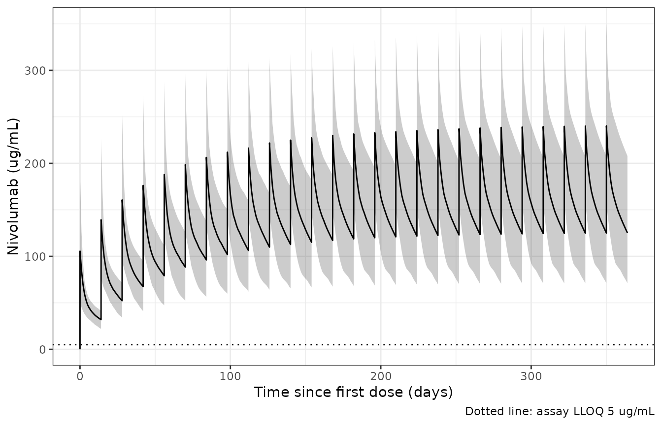
Simulated nivolumab serum concentrations after 240 mg every 2 weeks (median and 90% prediction interval, 200 virtual patients). Compare with the concentration range in Figure 3 of Tohi 2023 (a pcVPC of the observed data, which this simulation cannot reproduce point for point).
Replicating Figure 1: covariate effects on clearance
Figure 1 plots the individual post hoc CL against albumin, eGFR and
time since the first dose, with the final-model typical CL overlaid. The
typical curves are reproduced below from the model’s own cl
output.
typ <- rxode2::zeroRe(ui)
one_cl <- function(alb_gdL, egfr, time) {
  ev <- data.frame(id = seq_along(alb_gdL), time = time, amt = 0, evid = 0,
                   cmt = "central", ALB = alb_gdL * 10, CRCL = egfr)
  as.data.frame(rxode2::rxSolve(typ, ev, returnType = "data.frame"))$cl
}
alb_grid <- seq(2.5, 4.8, by = 0.05)
egfr_grid <- seq(29, 144, by = 1)
time_grid <- seq(0, 1217 * 24, by = 24)
fig1 <- bind_rows(
  tibble(panel = "A: albumin (g/dL)", x = alb_grid,
         cl = one_cl(alb_grid, rep(70, length(alb_grid)), rep(0, length(alb_grid)))),
  tibble(panel = "B: eGFR (mL/min/1.73 m^2)", x = egfr_grid,
         cl = one_cl(rep(3.6, length(egfr_grid)), egfr_grid, rep(0, length(egfr_grid)))),
  tibble(panel = "C: time since first dose (days)", x = time_grid / 24,
         cl = one_cl(rep(3.6, length(time_grid)), rep(70, length(time_grid)), time_grid))
)
#> ℹ omega/sigma items treated as zero: 'etalcl', 'etalvc'
#> Warning: multi-subject simulation without without 'omega'
#> ℹ omega/sigma items treated as zero: 'etalcl', 'etalvc'
#> Warning: multi-subject simulation without without 'omega'
#> ℹ omega/sigma items treated as zero: 'etalcl', 'etalvc'
#> Warning: multi-subject simulation without without 'omega'
ggplot(fig1, aes(x, cl)) +
  geom_line() +
  facet_wrap(~panel, scales = "free_x") +
  labs(x = NULL, y = "Typical CL (L/h)") +
  theme_bw()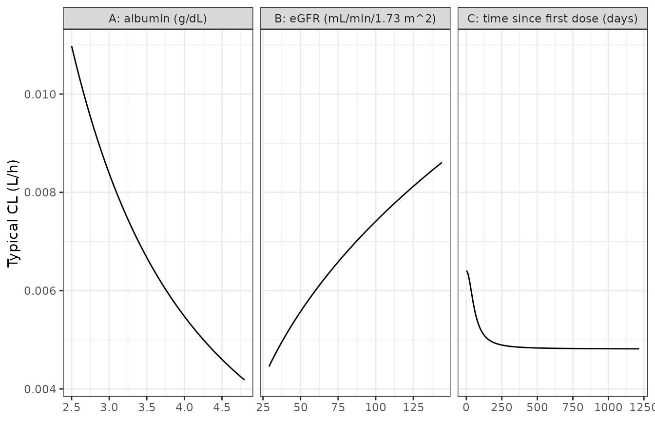
Typical nivolumab clearance versus albumin (at eGFR 70, t = 0), eGFR (at albumin 3.6 g/dL, t = 0) and time since the first dose (at the reference covariates). Replicates the solid lines of Figure 1A-C of Tohi 2023.
# The model's cl must equal the printed final CL equation evaluated by hand;
# both sides use the same numbers, so the bound is numerical tolerance only.
by_hand <- function(alb, egfr, t) {
  0.0064 * (alb / 3.6)^-1.48 * (egfr / 70)^0.411 *
    exp(-0.285 * t^2.02 / (1510^2.02 + t^2.02))
}
chk <- data.frame(alb = c(2.5, 3.6, 4.8, 3.6), egfr = c(30, 70, 144, 70),
                  t = c(0, 0, 2000, 8760))
chk$model <- mapply(one_cl, chk$alb, chk$egfr, chk$t)
#> ℹ omega/sigma items treated as zero: 'etalcl', 'etalvc'
#> ℹ omega/sigma items treated as zero: 'etalcl', 'etalvc'
#> ℹ omega/sigma items treated as zero: 'etalcl', 'etalvc'
#> ℹ omega/sigma items treated as zero: 'etalcl', 'etalvc'
chk$hand <- with(chk, by_hand(alb, egfr, t))
knitr::kable(chk, digits = 6)| alb | egfr | t | model | hand |
|---|---|---|---|---|
| 2.5 | 30 | 0 | 0.007750 | 0.007750 |
| 3.6 | 70 | 0 | 0.006400 | 0.006400 |
| 4.8 | 144 | 2000 | 0.004688 | 0.004688 |
| 3.6 | 70 | 8760 | 0.004851 | 0.004851 |
Replicating Figure S1: Monte Carlo trough concentrations
The authors simulated steady-state trough concentrations (Css,min) for 240 mg and 3 mg/kg every 2 weeks at albumin 2.5, 3.5 and 4.5 g/dL and eGFR 30, 60, 90 and 120 mL/min/1.73 m, and plotted them as boxplots (Figure S1). The medians below were digitised by the maintainers from Figure S1; the two extremes agree with the values stated in the Discussion (26.7 and 231.6 ug/mL), which are used directly for those two cells.
Because clearance keeps decreasing with time, the timing of “steady state” matters. The paper does not state it. Troughs are taken here at the end of the 26th dosing interval (one year, when the time effect on CL has reached 97% of its maximum) and, as a sensitivity, at the end of the 12th (24 weeks).
figS1_ref <- tribble(
  ~regimen,  ~alb, ~egfr, ~cmin_ref,
  "3 mg/kg", 2.5,  30,  61.7,
  "3 mg/kg", 2.5,  60,  41.2,
  "3 mg/kg", 2.5,  90,  31.9,
  "3 mg/kg", 2.5, 120,  26.7,
  "3 mg/kg", 3.5,  30, 113.2,
  "3 mg/kg", 3.5,  60,  81.0,
  "3 mg/kg", 3.5,  90,  65.2,
  "3 mg/kg", 3.5, 120,  55.8,
  "3 mg/kg", 4.5,  30, 174.0,
  "3 mg/kg", 4.5,  60, 126.0,
  "3 mg/kg", 4.5,  90, 102.6,
  "3 mg/kg", 4.5, 120,  93.3,
  "240 mg",  2.5,  30,  82.2,
  "240 mg",  2.5,  60,  55.3,
  "240 mg",  2.5,  90,  43.0,
  "240 mg",  2.5, 120,  37.1,
  "240 mg",  3.5,  30, 151.8,
  "240 mg",  3.5,  60, 106.7,
  "240 mg",  3.5,  90,  86.8,
  "240 mg",  3.5, 120,  75.1,
  "240 mg",  4.5,  30, 231.6,
  "240 mg",  4.5,  60, 169.3,
  "240 mg",  4.5,  90, 138.3,
  "240 mg",  4.5, 120, 123.7
) |>
  mutate(treatment = sprintf("%s, ALB %.1f, eGFR %d", regimen, alb, egfr))
n_per_arm <- 200
scen <- figS1_ref |>
  select(regimen, alb, egfr, treatment) |>
  mutate(scen = row_number())
wt_draw <- rtnorm(n_per_arm, 59.7, 12.3, 30, 120)

# One interval at the start and the 12th and 26th intervals are sampled
# densely enough for PKNCA; no dose is given after the 26th interval, so its
# end-of-interval sample is a clean trough.
nca_grid <- c(0, 0.5, 2, 6, 24, 48, 96, 168, 240, 336)
intervals_nca <- tibble(
  start = c(0, 11 * tau, 25 * tau),
  end = c(tau, 12 * tau, 26 * tau),
  window = c("Dose 1", "Dose 12", "Dose 26")
)
ev_s1 <- bind_rows(lapply(seq_len(nrow(scen)), function(k) {
  ids <- (k - 1) * n_per_arm + seq_len(n_per_arm)
  amt <- if (scen$regimen[k] == "240 mg") rep(240, n_per_arm) else 3 * wt_draw
  dose <- data.frame(id = rep(ids, each = n_dose), time = rep(dose_times, n_per_arm),
                     amt = rep(amt, each = n_dose), dur = 0.5, evid = 1)
  obs_t <- unique(unlist(lapply(intervals_nca$start, function(s) s + nca_grid)))
  obs <- data.frame(id = rep(ids, each = length(obs_t)),
                    time = rep(obs_t, n_per_arm), amt = 0, dur = 0, evid = 0)
  bind_rows(dose, obs) |>
    mutate(cmt = "central", ALB = scen$alb[k] * 10, CRCL = scen$egfr[k],
           treatment = scen$treatment[k])
})) |>
  arrange(id, time, desc(evid))

sim_s1 <- as.data.frame(rxode2::rxSolve(ui, ev_s1, keep = "treatment",
                                        returnType = "data.frame"))
trough <- sim_s1 |>
  filter(time %in% c(12 * tau, 26 * tau)) |>
  left_join(scen, by = "treatment") |>
  mutate(window = ifelse(time == 26 * tau, "Dose 26", "Dose 12"))

ggplot(filter(trough, window == "Dose 26"),
       aes(factor(egfr), Cc, fill = regimen)) +
  geom_boxplot(outlier.shape = NA) +
  geom_point(data = figS1_ref, aes(factor(egfr), cmin_ref, group = regimen),
             position = position_dodge(width = 0.75), shape = 4, size = 3) +
  facet_wrap(~ paste("ALB =", alb)) +
  coord_cartesian(ylim = c(0, 450)) +
  labs(x = "eGFR (mL/min/1.73 m^2)", y = "Css,min (ug/mL)", fill = "Dose") +
  theme_bw()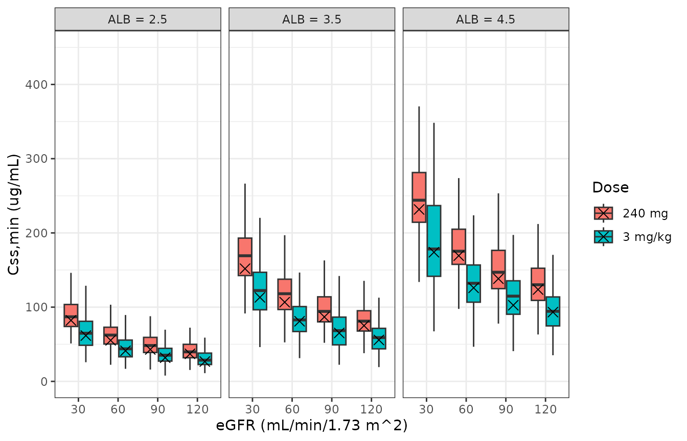
Simulated trough concentrations at the end of the 26th dosing interval by regimen, albumin and eGFR (boxes: 200 virtual patients per cell); crosses are the medians digitised from Figure S1 of Tohi 2023.
PKNCA validation
PKNCA computes Cmax, Cmin, AUC and average concentration over the
first, 12th and 26th dosing intervals for every Figure S1 cell. The
treatment grouping carries the regimen-albumin-eGFR cell.
Cmin of the first interval is the pre-dose zero; the later intervals’
Cmin is the trough at the end of the interval.
conc_s1 <- sim_s1 |>
  filter(!is.na(Cc)) |>
  select(id, time, Cc, treatment)
# Guarantee a time-zero record per subject for the first interval.
conc_s1 <- bind_rows(
  conc_s1,
  conc_s1 |> distinct(id, treatment) |> mutate(time = 0, Cc = 0)
) |>
  distinct(id, time, .keep_all = TRUE) |>
  arrange(id, time)

dose_s1 <- ev_s1 |>
  filter(evid == 1) |>
  select(id, time, amt, treatment)

conc_obj <- PKNCA::PKNCAconc(conc_s1, Cc ~ time | treatment + id,
                             concu = "ug/mL", timeu = "h")
dose_obj <- PKNCA::PKNCAdose(dose_s1, amt ~ time | treatment + id,
                             doseu = "mg")
intervals <- intervals_nca |>
  select(start, end) |>
  mutate(cmax = TRUE, cmin = TRUE, auclast = TRUE, cav = TRUE)
nca_res <- PKNCA::pk.nca(PKNCA::PKNCAdata(conc_obj, dose_obj, intervals = intervals))

nca_tab <- as.data.frame(nca_res) |>
  left_join(intervals_nca, by = c("start", "end")) |>
  filter(PPTESTCD %in% c("cmax", "cmin", "auclast", "cav")) |>
  group_by(treatment, window, PPTESTCD) |>
  summarise(median = median(PPORRES), .groups = "drop")

nca_tab |>
  filter(grepl("ALB 3.5, eGFR 60", treatment)) |>
  pivot_wider(names_from = PPTESTCD, values_from = median) |>
  rename(Treatment = treatment, Window = window,
         "Cmax (ug/mL)" = cmax, "Cmin (ug/mL)" = cmin,
         "AUC (ug*h/mL)" = auclast, "Cavg (ug/mL)" = cav) |>
knitr::kable(digits = 1, caption = "Median PKNCA results for the albumin 3.5 g/dL, eGFR 60 cells.")| Treatment | Window | AUC (ug*h/mL) | Cavg (ug/mL) | Cmax (ug/mL) | Cmin (ug/mL) |
|---|---|---|---|---|---|
| 240 mg, ALB 3.5, eGFR 60 | Dose 1 | 16253.0 | 48.4 | 105.2 | 0.0 |
| 240 mg, ALB 3.5, eGFR 60 | Dose 12 | 47205.1 | 140.5 | 218.5 | 108.2 |
| 240 mg, ALB 3.5, eGFR 60 | Dose 26 | 50848.2 | 151.3 | 229.1 | 118.0 |
| 3 mg/kg, ALB 3.5, eGFR 60 | Dose 1 | 11521.1 | 34.3 | 77.6 | 0.0 |
| 3 mg/kg, ALB 3.5, eGFR 60 | Dose 12 | 33867.8 | 100.8 | 157.2 | 75.7 |
| 3 mg/kg, ALB 3.5, eGFR 60 | Dose 26 | 36738.8 | 109.3 | 165.2 | 82.7 |
Comparison against Figure S1
sim_cmin_26 <- as.data.frame(nca_res) |>
  filter(PPTESTCD == "cmin", start == 25 * tau) |>
  select(treatment, PPTESTCD, PPORRES)
ref_cmin <- figS1_ref |>
  select(treatment, cmin = cmin_ref)

tbl <- nlmixr2lib::ncaComparisonTable(
  sim_cmin_26, ref_cmin,
  by = "treatment",
  units = c(cmin = "ug/mL"),
  tolerance_pct = 20
)
knitr::kable(tbl, caption = "Median trough at the end of the 26th dosing interval: Figure S1 of Tohi 2023 (digitised) vs this model.")| NCA parameter | treatment | Reference | Simulated | % diff |
|---|---|---|---|---|
| Cmin (ug/mL) | 3 mg/kg, ALB 2.5, eGFR 30 | 61.7 | 64.8 | +5.0% |
| Cmin (ug/mL) | 3 mg/kg, ALB 2.5, eGFR 60 | 41.2 | 43.8 | +6.4% |
| Cmin (ug/mL) | 3 mg/kg, ALB 2.5, eGFR 90 | 31.9 | 35.2 | +10.4% |
| Cmin (ug/mL) | 3 mg/kg, ALB 2.5, eGFR 120 | 26.7 | 28.6 | +6.9% |
| Cmin (ug/mL) | 3 mg/kg, ALB 3.5, eGFR 30 | 113 | 122 | +8.0% |
| Cmin (ug/mL) | 3 mg/kg, ALB 3.5, eGFR 60 | 81 | 82.7 | +2.1% |
| Cmin (ug/mL) | 3 mg/kg, ALB 3.5, eGFR 90 | 65.2 | 68.3 | +4.7% |
| Cmin (ug/mL) | 3 mg/kg, ALB 3.5, eGFR 120 | 55.8 | 58.9 | +5.6% |
| Cmin (ug/mL) | 3 mg/kg, ALB 4.5, eGFR 30 | 174 | 178 | +2.1% |
| Cmin (ug/mL) | 3 mg/kg, ALB 4.5, eGFR 60 | 126 | 132 | +4.6% |
| Cmin (ug/mL) | 3 mg/kg, ALB 4.5, eGFR 90 | 103 | 115 | +11.6% |
| Cmin (ug/mL) | 3 mg/kg, ALB 4.5, eGFR 120 | 93.3 | 94.2 | +1.0% |
| Cmin (ug/mL) | 240 mg, ALB 2.5, eGFR 30 | 82.2 | 86.9 | +5.7% |
| Cmin (ug/mL) | 240 mg, ALB 2.5, eGFR 60 | 55.3 | 62.3 | +12.6% |
| Cmin (ug/mL) | 240 mg, ALB 2.5, eGFR 90 | 43 | 48.3 | +12.3% |
| Cmin (ug/mL) | 240 mg, ALB 2.5, eGFR 120 | 37.1 | 39.7 | +7.1% |
| Cmin (ug/mL) | 240 mg, ALB 3.5, eGFR 30 | 152 | 169 | +11.2% |
| Cmin (ug/mL) | 240 mg, ALB 3.5, eGFR 60 | 107 | 118 | +10.5% |
| Cmin (ug/mL) | 240 mg, ALB 3.5, eGFR 90 | 86.8 | 94.2 | +8.5% |
| Cmin (ug/mL) | 240 mg, ALB 3.5, eGFR 120 | 75.1 | 81 | +7.9% |
| Cmin (ug/mL) | 240 mg, ALB 4.5, eGFR 30 | 232 | 243 | +5.0% |
| Cmin (ug/mL) | 240 mg, ALB 4.5, eGFR 60 | 169 | 175 | +3.4% |
| Cmin (ug/mL) | 240 mg, ALB 4.5, eGFR 90 | 138 | 147 | +6.1% |
| Cmin (ug/mL) | 240 mg, ALB 4.5, eGFR 120 | 124 | 130 | +5.1% |
attr(tbl, "footnote")
#> NULL
cmp <- trough |>
  group_by(treatment, regimen, alb, egfr, window) |>
  summarise(sim = median(Cc), .groups = "drop") |>
  left_join(select(figS1_ref, treatment, cmin_ref), by = "treatment") |>
  mutate(pct_diff = 100 * (sim / cmin_ref - 1))

cmp |>
  group_by(Window = window) |>
  summarise("Median % diff" = median(pct_diff),
            "Min % diff" = min(pct_diff),
            "Max % diff" = max(pct_diff), .groups = "drop") |>
knitr::kable(digits = 1, caption = "Simulated vs digitised Figure S1 medians, by the trough taken as steady state.")| Window | Median % diff | Min % diff | Max % diff |
|---|---|---|---|
| Dose 12 | -0.2 | -11.7 | 6.8 |
| Dose 26 | 6.4 | 1.2 | 12.8 |
cmp26 <- filter(cmp, window == "Dose 26")
stopifnot(
  # Structural: a mis-transcribed CL, exponent or reference value shifts the
  # whole grid by tens of percent.
  abs(median(cmp26$pct_diff)) < 20,
  quantile(abs(cmp26$pct_diff), 0.9) < 25
)
The relative effects stated in the Results can be recomputed from the simulated medians and compared with the published ranges.
med26 <- cmp26 |> select(regimen, alb, egfr, sim)
w <- med26 |> pivot_wider(names_from = regimen, values_from = sim)
reg_pct <- 100 * (w[["240 mg"]] / w[["3 mg/kg"]] - 1)

alb_w <- med26 |> pivot_wider(names_from = alb, values_from = sim, names_prefix = "alb")
alb_vs35 <- 100 * (1 - alb_w$alb2.5 / alb_w$alb3.5)
alb_vs45 <- 100 * (1 - alb_w$alb2.5 / alb_w$alb4.5)

egfr_w <- med26 |> pivot_wider(names_from = egfr, values_from = sim, names_prefix = "e")
e_vs60 <- 100 * (egfr_w$e30 / egfr_w$e60 - 1)
e_vs90 <- 100 * (egfr_w$e30 / egfr_w$e90 - 1)
e_vs120 <- 100 * (egfr_w$e30 / egfr_w$e120 - 1)

ratio_tab <- tibble(
  Comparison = c("240 mg vs 3 mg/kg, % higher",
                 "ALB 2.5 vs 3.5 g/dL, % lower",
                 "ALB 2.5 vs 4.5 g/dL, % lower",
                 "eGFR 30 vs 60, % higher",
                 "eGFR 30 vs 90, % higher",
                 "eGFR 30 vs 120, % higher"),
  Published = c("32.2-38.3", "45.7-51.9", "64.5-71.4", "36.6-49.3", "67.3-93.0", "85.9-129.8"),
  Simulated = sapply(list(reg_pct, alb_vs35, alb_vs45, e_vs60, e_vs90, e_vs120),
                     function(x) sprintf("%.1f-%.1f", min(x), max(x)))
)
knitr::kable(ratio_tab, caption = "Relative differences in median Css,min (Tohi 2023 Results, 'Monte Carlo Simulation Analysis') vs this model.")| Comparison | Published | Simulated |
|---|---|---|
| 240 mg vs 3 mg/kg, % higher | 32.2-38.3 | 28.0-42.6 |
| ALB 2.5 vs 3.5 g/dL, % lower | 45.7-51.9 | 47.0-51.5 |
| ALB 2.5 vs 4.5 g/dL, % lower | 64.5-71.4 | 63.6-69.7 |
| eGFR 30 vs 60, % higher | 36.6-49.3 | 34.9-47.8 |
| eGFR 30 vs 90, % higher | 67.3-93.0 | 55.3-83.9 |
| eGFR 30 vs 120, % higher | 85.9-129.8 | 87.5-126.9 |
# The published ranges come from 1000-patient simulations; allow a few
# percentage points of Monte Carlo noise around each range.
stopifnot(
  median(reg_pct) > 25, median(reg_pct) < 45,
  median(alb_vs35) > 40, median(alb_vs35) < 58,
  median(alb_vs45) > 58, median(alb_vs45) < 78,
  median(e_vs120) > 75, median(e_vs120) < 140
)
Assumptions and deviations
Errata and readings that required arbitration
-
T50 printed as 1501 h in the final CL equation.
Methods (“T50 (1510 h)”) and Table 2 (“1510 (FIX)”) both give 1510 h,
and the value is stated to be taken unchanged from Osawa et al. The
final equation in the Results prints
1501^2.02, read here as a transposition. The model uses 1510 h; the two values change CL by less than 0.5% at any time. - Minus signs in the PDF text layer. The PDF text layer renders the minus sign as “2” (e.g. “2 1.48”, “2 0.285”); the signs were confirmed on the typeset page. The negative albumin exponent also agrees with the text (“ALB levels negatively correlated with nivolumab CL”).
Assumptions made because the paper does not say
- IIV scale. Table 2 reports IIV as CV%. The variances use omega = log(1 + CV); reading CV% as 100 x omega instead would give 0.0376 and 0.214, within the bootstrap 95% CIs either way.
- Infusion duration. Not reported; 30 minutes is used.
-
Time origin. The time-varying CL uses time since
the first dose; the model reads it from rxode2’s
t, so the first dose must be at time 0. - Steady state in the Monte Carlo simulation. Not defined in the paper. The trough at the end of the 26th interval (one year) is the primary comparison; its medians run 1-13% above the digitised Figure S1 medians (median +6%). The 24-week trough, shown as a sensitivity, agrees with Figure S1 to within -12% to +7% (median 0%), so the authors’ steady state may be earlier than one year. The relative effects of regimen, albumin and eGFR match the published ranges at either time. No parameter was adjusted to close the gap.
- Covariate distributions. Baseline albumin and eGFR are drawn from normal distributions with the Table S3 means and SDs, truncated to the Table 1 ranges, and held constant over time (Table S3 shows no systematic change).
-
Albumin units. The published coefficient and the
reference 3.6 are in g/dL; the model takes the canonical
ALBcolumn in g/L and converts.
Session info
sessionInfo()
#> R version 4.6.1 (2026-06-24)
#> Platform: x86_64-pc-linux-gnu
#> Running under: Ubuntu 24.04.5 LTS
#>
#> Matrix products: default
#> BLAS:   /usr/lib/x86_64-linux-gnu/openblas-pthread/libblas.so.3
#> LAPACK: /usr/lib/x86_64-linux-gnu/openblas-pthread/libopenblasp-r0.3.26.so;  LAPACK version 3.12.0
#>
#> locale:
#>  [1] LC_CTYPE=C.UTF-8       LC_NUMERIC=C           LC_TIME=C.UTF-8
#>  [4] LC_COLLATE=C.UTF-8     LC_MONETARY=C.UTF-8    LC_MESSAGES=C.UTF-8
#>  [7] LC_PAPER=C.UTF-8       LC_NAME=C              LC_ADDRESS=C
#> [10] LC_TELEPHONE=C         LC_MEASUREMENT=C.UTF-8 LC_IDENTIFICATION=C
#>
#> time zone: UTC
#> tzcode source: system (glibc)
#>
#> attached base packages:
#> [1] stats     graphics  grDevices utils     datasets  methods   base
#>
#> other attached packages:
#> [1] ggplot2_4.0.3         tidyr_1.3.2           dplyr_1.2.1
#> [4] rxode2_5.1.8          PKNCA_0.12.1          nlmixr2lib_0.3.2.9000
#>
#> loaded via a namespace (and not attached):
#>  [1] gtable_0.3.6        xfun_0.62           bslib_0.12.0
#>  [4] rxode2lincmt_0.1.0  lattice_0.22-9      vctrs_0.7.3
#>  [7] tools_4.6.1         generics_0.1.4      parallel_4.6.1
#> [10] tibble_3.3.1        symengine_0.2.14    pkgconfig_2.0.3
#> [13] data.table_1.18.6.1 checkmate_2.3.4     RColorBrewer_1.1-3
#> [16] S7_0.2.2            desc_1.4.3          lifecycle_1.0.5
#> [19] compiler_4.6.1      farver_2.1.2        textshaping_1.0.5
#> [22] fontawesome_0.5.3   htmltools_0.5.9     sys_3.4.3
#> [25] sass_0.4.10         yaml_2.3.12         pillar_1.11.1
#> [28] pkgdown_2.2.1       crayon_1.5.3        jquerylib_0.1.4
#> [31] whisker_0.4.1       openssl_2.4.2       cachem_1.1.0
#> [34] nlme_3.1-169        tidyselect_1.2.1    digest_0.6.39
#> [37] lotri_1.0.5         purrr_1.2.2         labeling_0.4.3
#> [40] rxode2ll_2.0.18     fastmap_1.2.0       grid_4.6.1
#> [43] cli_3.6.6           dparser_1.3.1-14    magrittr_2.0.5
#> [46] withr_3.0.3         scales_1.4.0        backports_1.5.1
#> [49] rmarkdown_2.32      otel_0.2.0          askpass_1.2.1
#> [52] ragg_1.5.2          memoise_2.0.1       evaluate_1.0.5
#> [55] knitr_1.52          rex_1.2.2           PreciseSums_0.7
#> [58] rlang_1.3.0         downlit_0.4.5       Rcpp_1.1.2
#> [61] glue_1.8.1          xml2_1.6.0          jsonlite_2.0.0
#> [64] R6_2.6.1            systemfonts_1.3.2   fs_2.1.0