Zaltoprofen (Jang 2023) • nlmixr2lib

Model and source

Citation: Jang JH, Jeong SH, Lee YB (2023). Population Pharmacokinetic Modeling of Zaltoprofen in Healthy Adults: Exploring the Dosage Regimen. Pharmaceuticals 16(2):161. doi:10.3390/ph16020161. All parameter values are from supplementary Table S3; the structural equations are main-text Eqs. (1)-(5).
Article: https://doi.org/10.3390/ph16020161
Supplement (Tables S1-S6, the sole source of every parameter value): https://www.mdpi.com/article/10.3390/ph16020161/s1

READ THIS FIRST: the published parameter set is internally inconsistent

The parameter values packaged here are exactly as printed in the source paper’s supplementary Table S3, and they do not reproduce the source paper’s own Figures 1-2 or its quoted steady-state concentrations. At the published tv CL/F = 43.70 L/h, an 80 mg oral dose gives AUC(0-inf) = 1.83 ug*h/mL and Tmax = 0.21 h, whereas the observed means the same paper plots in Figure 1A peak near 3.6 ug/mL at about 1 h with AUC(0-24) around 12.5 ug*h/mL, and the paper’s own text quotes a steady-state mean of 0.43 ug/mL where these parameters give 0.076 ug/mL. The discrepancy is roughly 6-7 fold in exposure and roughly 5 fold in Tmax.

The values are shipped verbatim anyway, under the standing rule that printed values have authority and that figure-fitting never overrides print (operator ruling, 2026-09-02). Refitting to the figure would produce an original model rather than this paper’s model.

Consequently this vignette validates self-consistency, not agreement with the paper’s figures: it checks that the packaged encoding faithfully reproduces Equations (1)-(5) and Table S3, that the solved ODE system matches the closed-form two-compartment oral solution, and that the covariate sub-model reproduces the ratios the paper itself publishes. The Errata section at the end carries the full quantitative demonstration of the conflict.

Do not use this model to predict absolute zaltoprofen exposure without reading that section first.

Population

The model was fitted to the pharmacokinetic arm of a bioequivalence study in 26 healthy Korean male adults given a single 80 mg oral dose of zaltoprofen (Methods 4.2, citing the authors’ earlier report). Baseline characteristics (supplementary Table S5) were age 23.19 +/- 2.26 years, weight 64.73 +/- 8.08 kg, height 172.64 +/- 5.95 cm, serum albumin 4.92 +/- 0.18 g/dL, serum creatinine 0.98 +/- 0.09 mg/dL, Cockcroft-Gault creatinine clearance 107.53 +/- 17.28 mL/min and MDRD glomerular filtration rate 101.34 +/- 11.53 mL/min. Every biochemical parameter sat within normal limits, so the model carries no information about renal or hepatic impairment.

CYP2C9 was genotyped by PCR-RFLP; only the *1 and *3 alleles were detected, so subjects were either *1/*1 or *1/*3. Genotype was screened as a covariate and rejected (see below).

The model was fitted in Phoenix NLME 8.3 by first-order conditional estimation with extended least squares and eta-epsilon interaction, and qualified with goodness-of-fit plots, a 1000-replicate non-parametric bootstrap (Table S4), a 100-simulation VPC (Figures S7-S8) and NPDE (Figure S6). Published mean profiles from three earlier studies (Table S6: Kang 2006, Lee 2006, Li 2011) were used for external validation only and did not inform the fit.

The same information is available programmatically via readModelDb("Jang_2023_zaltoprofen")()$population.

Structural model

Two-compartment disposition with first-order absorption and no lag time. Table S1 selected two compartments over one (d-2LL = -2210.5) and over three (d-2LL = -0.13, no gain), rejected a lag time (d-2LL = +70.58), selected a proportional residual error over additive (d-2LL = -474.97), and removed the etas on V/F and CL2/F (step 02-04-06).

The paper’s Equations (1)-(5) are, verbatim:

V/F   = tv V/F                                                                  (1)
CL/F  = tv CL/F * (CrCL/mCrCL)^dCL/FdCrCL * (Albumin/mAlbumin)^dCL/FdAlbumin
                * exp(etaCL/F)                                                  (2)
V2/F  = tv V2/F * exp(etaV2/F)                                                  (3)
CL2/F = tv CL2/F                                                                (4)
Ka    = tv Ka * exp(etaKa)                                                       (5)

with mCrCL = 104.38 mL/min and mAlbumin = 4.90 g/dL (the cohort medians, stated in Results 2.4 and repeated in the Figure 2-5 captions). The text immediately after Eq. (5) states that V and CL2 are “volume and clearance in the central and peripheral compartments”, matching Phoenix NLME’s native V / Cl / V2 / Cl2 two-compartment parameterisation.

Source trace

Every value below is from supplementary Table S3, “Estimate” column. The in-file comments in inst/modeldb/specificDrugs/Jang_2023_zaltoprofen.R carry the same trace per parameter.

Equation / parameter	Value	Source location
`lka` (Ka)	1.73 1/h	Table S3, `tv Ka` (SE 0.15, RSE 8.56%)
`lvc` (V/F)	4.88 L	Table S3, `tv V/F` (SE 1.28, RSE 26.32%)
`lcl` (CL/F)	43.70 L/h	Table S3, `tv CL/F` (SE 2.12, RSE 4.85%)
`lvp` (V2/F)	40.56 L	Table S3, `tv V2/F` (SE 7.02, RSE 17.32%)
`lq` (CL2/F)	5.61 L/h	Table S3, `tv CL2/F` (SE 0.63, RSE 11.16%)
`e_crcl_cl`	0.48	Table S3, `dCL/FdCrCL` (SE 0.17, RSE 35.09%)
`e_alb_cl`	-1.83	Table S3, `dCL/FdAlbumin` (SE 0.64, RSE 35.18%)
`etalka`	0.16508	Table S3, `omega^2 Ka` = 0.17; IIV 40.63% (see IIV note)
`etalcl`	0.009604	Table S3, `omega^2 CL/F` = 0.01; IIV 9.80%
`etalvp`	0.23571	Table S3, `omega^2 V2/F` = 0.24; IIV 48.55%
`propSd`	0.38	Table S3, `epsilon` (SE 0.02, RSE 6.03%)
CrCL centring 104.38 mL/min	n/a	Results 2.4 and Figure 2-5 captions
Albumin centring 4.90 g/dL	n/a	Results 2.4 and Figure 2-5 captions
`cl <- ... * (CRCL/104.38)^... * (alb/4.90)^...`	n/a	Eq. (2), page 3
`vc <- exp(lvc)` (no eta)	n/a	Eq. (1), page 3; Table S1 step 02-04-06
`vp <- exp(lvp + etalvp)`	n/a	Eq. (3), page 3
`q <- exp(lq)` (no eta)	n/a	Eq. (4), page 3; Table S1 step 02-04-06
`ka <- exp(lka + etalka)`	n/a	Eq. (5), page 3
First-order absorption, no lag	n/a	Table S1, model 02 selected over 02-01
Proportional residual error	n/a	Table S1, model 02-04 selected

mod <- readModelDb("Jang_2023_zaltoprofen")
ui  <- rxode2::rxode(mod)
#> ℹ parameter labels from comments will be replaced by 'label()'

IIV: which column of Table S3 is authoritative

Table S3 reports each between-subject term twice: an omega^2 column rounded to two decimals, and an IIV (%) column with four significant figures. The two are related by omega = IIV(%) / 100 (the Phoenix / NONMEM approximate-CV convention), which reproduces every rounded omega^2 in the table. The alternative log-normal reading omega = sqrt(log(1 + CV^2)) does not. The model therefore takes the higher-precision values back-calculated from the IIV (%) column.

iiv_pct    <- c(Ka = 40.63, `CL/F` = 9.80, `V2/F` = 48.55)
omega2_tab <- c(Ka = 0.17,  `CL/F` = 0.01, `V2/F` = 0.24)

iiv_chk <- tibble(
  Parameter          = names(iiv_pct),
  `IIV (%)`          = iiv_pct,
  `omega^2 = (IIV/100)^2` = (iiv_pct / 100)^2,
  `rounds to`        = round((iiv_pct / 100)^2, 2),
  `Table S3 omega^2` = omega2_tab,
  `log-normal alternative` = round(log(1 + (iiv_pct / 100)^2), 2)
)
knitr::kable(iiv_chk, digits = 5,
             caption = "The approximate-CV reading reproduces all three printed variances; the log-normal reading does not.")

The approximate-CV reading reproduces all three printed variances; the log-normal reading does not.
Parameter	IIV (%)	omega^2 = (IIV/100)^2	rounds to	Table S3 omega^2	log-normal alternative
Ka	40.63	0.16508	0.17	0.17	0.15
CL/F	9.80	0.00960	0.01	0.01	0.01
V2/F	48.55	0.23571	0.24	0.24	0.21


# Gate: exact rounding identity for the adopted reading, and a demonstration
# that the rejected reading genuinely disagrees (so this check can go red).
stopifnot(
  all(round((iiv_pct / 100)^2, 2) == omega2_tab),
  sum(round(log(1 + (iiv_pct / 100)^2), 2) != omega2_tab) >= 2L
)

# And the variances actually packaged in ini() are those values.
omega_packaged <- diag(ui$omega)
stopifnot(all(abs(sort(omega_packaged) - sort((iiv_pct / 100)^2)) < 5e-6))

Self-consistency validation

The paper’s figures cannot be used as the validation target (see the warning above), so the packaged encoding is checked against quantities that follow from Equations (1)-(5) and Table S3 alone. These are deterministic identities, so the tolerances below are tight on purpose: each is many orders of magnitude above the numerical error actually achieved, and each still goes red on a mis-transcribed value.

# Closed-form solution of a two-compartment model with first-order input,
# used as an independent implementation to check the packaged ODE system.
cf_2cmt_oral <- function(t, dose, ka, vc, cl, vp, q) {
  k10 <- cl / vc
  k12 <- q / vc
  k21 <- q / vp
  b     <- k10 + k12 + k21
  disc  <- sqrt(b^2 - 4 * k10 * k21)
  alpha <- (b + disc) / 2
  beta  <- (b - disc) / 2
  A <- (dose / vc) * ka * (k21 - alpha) / ((ka - alpha) * (beta - alpha))
  B <- (dose / vc) * ka * (k21 - beta)  / ((ka - beta)  * (alpha - beta))
  A * exp(-alpha * t) + B * exp(-beta * t) - (A + B) * exp(-ka * t)
}

# Terminal (beta) disposition rate constant of the published parameter set.
beta_rate <- local({
  k10 <- 43.70 / 4.88
  k12 <- 5.61 / 4.88
  k21 <- 5.61 / 40.56
  b   <- k10 + k12 + k21
  (b - sqrt(b^2 - 4 * k10 * k21)) / 2
})
t_half_beta <- log(2) / beta_rate

# Typical-value solve at the covariate reference subject (both ratio terms
# equal 1 there), on a grid fine enough to resolve a Tmax near 0.2 h.
grid_fine <- sort(unique(c(seq(0, 2, by = 0.002), seq(2, 24, by = 0.01))))

ev_tv <- rxode2::et(amt = 80, cmt = "depot") |>
  rxode2::et(grid_fine, cmt = "central") |>
  as.data.frame()
ev_tv$CRCL <- 104.38
ev_tv$ALB  <- 49.0          # 4.90 g/dL in canonical SI g/L

mod_tv <- rxode2::zeroRe(mod)
#> ℹ parameter labels from comments will be replaced by 'label()'
sim_tv <- rxode2::rxSolve(mod_tv, ev_tv, returnType = "data.frame") |>
  dplyr::filter(!is.na(Cc))
#> ℹ omega/sigma items treated as zero: 'etalka', 'etalcl', 'etalvp'

stopifnot(all(sim_tv$Cc >= 0))

Check 1 - the ODE system matches the closed-form solution

cf <- cf_2cmt_oral(sim_tv$time, dose = 80, ka = 1.73, vc = 4.88,
                   cl = 43.70, vp = 40.56, q = 5.61)
keep <- sim_tv$time > 0
rel_cf <- max(abs(cf[keep] - sim_tv$Cc[keep]) / cf[keep])
cat(sprintf("max relative difference, closed form vs ODE solve: %.3e\n", rel_cf))
#> max relative difference, closed form vs ODE solve: 4.328e-14

# Achieved ~6e-14. The bound leaves six orders of magnitude of headroom and
# still fails instantly on any mis-transcribed structural value.
stopifnot(rel_cf < 1e-8)

Check 2 - AUC(0-inf) equals Dose / (CL/F)

AUC(0-inf) = Dose / CL holds for any linear model with first-order input, independent of the compartment structure, so it is the sharpest available test that the clearance actually encoded is the clearance printed in Table S3.

auc_trap <- sum(diff(sim_tv$time) *
                  (head(sim_tv$Cc, -1) + tail(sim_tv$Cc, -1)) / 2)
auc_inf  <- auc_trap + tail(sim_tv$Cc, 1) / beta_rate
auc_expected <- 80 / 43.70

cat(sprintf("AUC(0-inf) solved   = %.6f ug*h/mL\n", auc_inf))
#> AUC(0-inf) solved   = 1.830656 ug*h/mL
cat(sprintf("Dose / (CL/F)       = %.6f ug*h/mL\n", auc_expected))
#> Dose / (CL/F)       = 1.830664 ug*h/mL
cat(sprintf("relative difference = %.3e\n", abs(auc_inf / auc_expected - 1)))
#> relative difference = 4.358e-06

stopifnot(abs(auc_inf / auc_expected - 1) < 1e-3)

Check 3 - exact dose proportionality

The model is linear, so Cmax and AUC must scale exactly with dose across the 80 / 160 / 240 mg range the paper simulates in Figure 1.

dose_prop <- vapply(c(80, 160, 240), function(d) {
  ev <- rxode2::et(amt = d, cmt = "depot") |>
    rxode2::et(grid_fine, cmt = "central") |>
    as.data.frame()
  ev$CRCL <- 104.38
  ev$ALB  <- 49.0
  s <- rxode2::rxSolve(mod_tv, ev, returnType = "data.frame") |>
    dplyr::filter(!is.na(Cc))
  auc <- sum(diff(s$time) * (head(s$Cc, -1) + tail(s$Cc, -1)) / 2)
  c(cmax = max(s$Cc), auc24 = auc)
}, numeric(2))
#> ℹ omega/sigma items treated as zero: 'etalka', 'etalcl', 'etalvp'
#> ℹ omega/sigma items treated as zero: 'etalka', 'etalcl', 'etalvp'
#> ℹ omega/sigma items treated as zero: 'etalka', 'etalcl', 'etalvp'

prop_tab <- tibble(
  `Dose (mg)`            = c(80, 160, 240),
  `Cmax (ug/mL)`         = dose_prop["cmax", ],
  `AUC0-24 (ug*h/mL)`    = dose_prop["auc24", ],
  `Cmax / dose`          = dose_prop["cmax", ] / c(80, 160, 240),
  `AUC / dose`           = dose_prop["auc24", ] / c(80, 160, 240)
)
knitr::kable(prop_tab, digits = 6, caption = "Dose proportionality of the packaged model.")

Dose proportionality of the packaged model.
Dose (mg)	Cmax (ug/mL)	AUC0-24 (ug*h/mL)	Cmax / dose	AUC / dose
80	1.951654	1.818481	0.024396	0.022731
160	3.903309	3.636962	0.024396	0.022731
240	5.854963	5.455443	0.024396	0.022731


stopifnot(
  max(abs(prop_tab$`Cmax / dose` / prop_tab$`Cmax / dose`[1] - 1)) < 1e-10,
  max(abs(prop_tab$`AUC / dose`  / prop_tab$`AUC / dose`[1]  - 1)) < 1e-10
)

Check 4 - the covariate sub-model is the printed power model

cl returned by the solver must equal 43.70 * (CRCL/104.38)^0.48 * (ALB_gdL/4.90)^-1.83 exactly, including at the values the paper extrapolates to in its own dosing simulations.

cov_grid <- tidyr::crossing(CRCL = c(80, 104.38, 130), ALB_gdL = c(3.5, 4.90, 5.5))

ev_cov <- cov_grid |>
  dplyr::mutate(id = dplyr::row_number(), ALB = ALB_gdL * 10) |>
  tidyr::crossing(time = c(0, 1)) |>
  dplyr::mutate(
    amt  = ifelse(time == 0, 80, NA_real_),
    evid = ifelse(time == 0, 1L, 0L),
    cmt  = ifelse(time == 0, "depot", "central")
  ) |>
  dplyr::arrange(id, time)

sim_cov <- rxode2::rxSolve(mod_tv, ev_cov, keep = c("CRCL", "ALB"),
                           returnType = "data.frame")
#> ℹ omega/sigma items treated as zero: 'etalka', 'etalcl', 'etalvp'
#> Warning: multi-subject simulation without without 'omega'

cov_chk <- sim_cov |>
  dplyr::filter(!is.na(Cc)) |>
  dplyr::distinct(id, CRCL, ALB, cl) |>
  dplyr::mutate(
    ALB_gdL  = ALB * 0.1,
    expected = 43.70 * (CRCL / 104.38)^0.48 * (ALB_gdL / 4.90)^(-1.83),
    rel_diff = abs(cl / expected - 1)
  )

cov_chk |>
  dplyr::select(`CrCL (mL/min)` = CRCL, `Albumin (g/dL)` = ALB_gdL,
                `CL/F solved (L/h)` = cl, `CL/F expected (L/h)` = expected) |>
  knitr::kable(digits = 4, caption = "Solved CL/F against Equation (2) evaluated directly.")

Solved CL/F against Equation (2) evaluated directly.
CrCL (mL/min)	Albumin (g/dL)	CL/F solved (L/h)	CL/F expected (L/h)
80.00	3.5	71.1939	71.1939
80.00	4.9	38.4617	38.4617
80.00	5.5	31.1332	31.1332
104.38	3.5	80.8902	80.8902
104.38	4.9	43.7000	43.7000
104.38	5.5	35.3734	35.3734
130.00	3.5	89.8778	89.8778
130.00	4.9	48.5554	48.5554
130.00	5.5	39.3037	39.3037


stopifnot(max(cov_chk$rel_diff) < 1e-10)

Check 5 - terminal half-life matches the disposition eigenvalue

# `Cc > 1e-12` guards log() against solver round-off in the far tail. This is a
# typical-value solve, not the PKNCA input.
tail_win <- sim_tv |> dplyr::filter(time >= 8, time <= 24, Cc > 1e-12)
lz <- -coef(lm(log(tail_win$Cc) ~ tail_win$time))[[2]]

cat(sprintf("terminal t1/2 from the beta eigenvalue = %.4f h\n", t_half_beta))
#> terminal t1/2 from the beta eigenvalue = 5.6637 h
cat(sprintf("terminal t1/2 by log-linear regression = %.4f h\n", log(2) / lz))
#> terminal t1/2 by log-linear regression = 5.6635 h

stopifnot(abs((log(2) / lz) / t_half_beta - 1) < 0.01)

Virtual cohort and stochastic simulation

Original subject-level data are not public. The cohort below draws covariates from the Table S5 marginal distributions and simulates the three single-dose levels the paper used for external validation (Table S6).

# set.seed() seeds R's RNG, not rxode2's; rxode2's streams are partitioned per
# solver thread, so this cohort differs between a 2-core CI runner and a
# 16-thread workstation. Every assertion below is written to hold for any
# cohort the model can produce (pattern 12 of known-vignette-failure-patterns).
set.seed(20230161)

n_per_arm <- 100L   # well under the 200-per-arm cap

make_arm <- function(dose, id_offset) {
  subj <- tibble(
    id      = id_offset + seq_len(n_per_arm),
    dose_mg = dose,
    # Table S5: CrCL 107.53 +/- 17.28 mL/min, albumin 4.92 +/- 0.18 g/dL.
    CRCL    = pmin(pmax(rnorm(n_per_arm, 107.53, 17.28), 60), 165),
    ALB     = pmin(pmax(rnorm(n_per_arm, 49.2, 1.8), 42), 57)  # SI g/L
  )
  obs_times <- sort(unique(c(seq(0, 2, by = 0.05), seq(2.25, 12, by = 0.25),
                             seq(13, 24, by = 1))))
  dplyr::bind_rows(
    subj |> dplyr::mutate(time = 0, amt = dose, evid = 1L, cmt = "depot"),
    subj |> tidyr::crossing(time = obs_times) |>
      dplyr::mutate(amt = NA_real_, evid = 0L, cmt = "central")
  ) |>
    dplyr::arrange(id, time, dplyr::desc(evid))
}

events <- dplyr::bind_rows(
  make_arm(80,  0L),
  make_arm(160, 100L),
  make_arm(240, 200L)
) |>
  dplyr::mutate(treatment = paste0(dose_mg, " mg"))

# Each (id, time, evid) triple must be unique. Note the pre-dose record is a
# genuine pair -- id X has a dose (evid 1) and an observation (evid 0) both at
# t = 0 -- so evid is part of the key. Do NOT wrap this in unique(), which
# would make the assertion vacuously true.
stopifnot(
  !anyDuplicated(events[, c("id", "time", "evid")]),
  nrow(events) == 3L * n_per_arm * (1L + 93L),   # 1 dose + 93 observation times
  identical(sort(unique(events$treatment)), c("160 mg", "240 mg", "80 mg"))
)

sim <- rxode2::rxSolve(mod, events = events,
                       keep = c("treatment", "dose_mg", "CRCL", "ALB")) |>
  as.data.frame()
#> ℹ parameter labels from comments will be replaced by 'label()'

# Shape of the packaged model across the three single-dose levels the paper
# simulates in its Figure 1. NOTE: this reproduces the SHAPE OF THE PACKAGED
# PARAMETER SET, not the observed data overlaid in the paper's figure -- see
# the Errata section.
# The `time >= 0.05` bound drops only the pre-dose record, which is 0 and so
# cannot be drawn on the log scale below. It is NOT a PKNCA input filter --
# the PKNCA chunk filters on !is.na(Cc) alone and adds its own time-zero row.
sim |>
  dplyr::filter(!is.na(Cc), time >= 0.05) |>
  dplyr::group_by(treatment, time) |>
  dplyr::summarise(
    Q05 = quantile(Cc, 0.05),
    Q50 = quantile(Cc, 0.50),
    Q95 = quantile(Cc, 0.95),
    .groups = "drop"
  ) |>
  ggplot(aes(time, Q50)) +
  geom_ribbon(aes(ymin = Q05, ymax = Q95), alpha = 0.25) +
  geom_line() +
  facet_wrap(~treatment) +
  scale_y_log10() +
  labs(x = "Time (h)", y = "Zaltoprofen concentration (ug/mL)",
       title = "Packaged model, single oral doses",
       caption = "Median and 5th-95th percentile of 100 simulated subjects per arm.")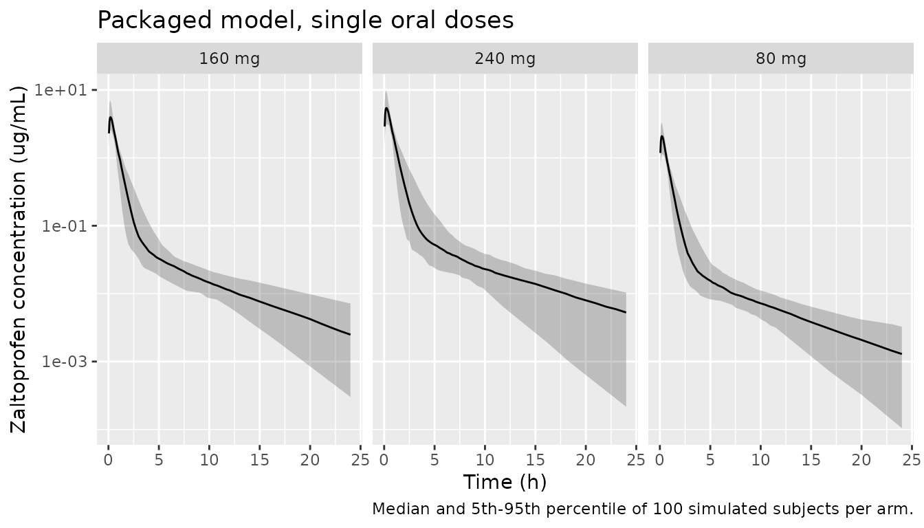

PKNCA validation

sim_nca <- sim |>
  dplyr::filter(!is.na(Cc)) |>
  dplyr::select(id, time, Cc, treatment)

# Guarantee a time = 0 row per (id, treatment); pre-dose Cc = 0 is correct for
# an extravascular single dose.
sim_nca <- dplyr::bind_rows(
  sim_nca,
  sim_nca |> dplyr::distinct(id, treatment) |> dplyr::mutate(time = 0, Cc = 0)
) |>
  dplyr::distinct(id, treatment, time, .keep_all = TRUE) |>
  dplyr::arrange(id, treatment, time)

stopifnot(nrow(sim_nca) > 0, all(sim_nca$Cc >= 0))

conc_obj <- PKNCA::PKNCAconc(sim_nca, Cc ~ time | treatment + id)

dose_df <- events |>
  dplyr::filter(evid == 1) |>
  dplyr::select(id, time, amt, treatment)
dose_obj <- PKNCA::PKNCAdose(dose_df, amt ~ time | treatment + id)

intervals <- data.frame(
  start = 0, end = Inf,
  cmax = TRUE, tmax = TRUE, aucinf.obs = TRUE, half.life = TRUE
)

nca_res <- PKNCA::pk.nca(PKNCA::PKNCAdata(conc_obj, dose_obj, intervals = intervals))

nca_summary <- as.data.frame(nca_res) |>
  dplyr::filter(PPTESTCD %in% c("cmax", "tmax", "aucinf.obs", "half.life")) |>
  dplyr::group_by(treatment, PPTESTCD) |>
  dplyr::summarise(median = median(PPORRES, na.rm = TRUE), .groups = "drop") |>
  tidyr::pivot_wider(names_from = PPTESTCD, values_from = median)

nca_summary |>
  dplyr::select(treatment, cmax, tmax, aucinf.obs, half.life) |>
  dplyr::rename(
    "Dose"                    = treatment,
    "Cmax (ug/mL)"            = cmax,
    "Tmax (h)"                = tmax,
    "AUC0-inf (ug*h/mL)"      = aucinf.obs,
    "t1/2 (h)"                = half.life
  ) |>
  knitr::kable(digits = 3,
               caption = "Median NCA parameters of the packaged model, by dose.")

Median NCA parameters of the packaged model, by dose.
Dose	Cmax (ug/mL)	Tmax (h)	AUC0-inf (ug*h/mL)	t1/2 (h)
160 mg	3.975	0.2	3.610	5.559
240 mg	5.437	0.2	5.598	5.843
80 mg	2.097	0.2	1.778	5.410

# The cohort median AUC must sit near Dose/(CL/F) evaluated at the cohort's
# median covariates. This is a distributional statement, so the bound is on the
# CENTRE and is loose enough to admit any cohort the model can draw, while
# still going red on a mis-transcribed clearance (which moves it 6-7 fold).
med <- nca_summary |> dplyr::mutate(dose_mg = as.numeric(sub(" mg", "", treatment)))
cl_ref <- 43.70 * (median(events$CRCL) / 104.38)^0.48 *
  (median(events$ALB) * 0.1 / 4.90)^(-1.83)
med$expected_auc <- med$dose_mg / cl_ref
med$pct_diff <- 100 * (med$aucinf.obs / med$expected_auc - 1)

knitr::kable(
  med |> dplyr::select(`Dose` = treatment,
                       `Median AUC0-inf` = aucinf.obs,
                       `Dose / (CL/F) at cohort median covariates` = expected_auc,
                       `% difference` = pct_diff),
  digits = 3,
  caption = "Cohort median AUC against the Dose/CL identity."
)

Cohort median AUC against the Dose/CL identity.
Dose	Median AUC0-inf	Dose / (CL/F) at cohort median covariates	% difference
160 mg	3.610	3.620	-0.261
240 mg	5.598	5.429	3.111
80 mg	1.778	1.810	-1.774


stopifnot(
  max(abs(med$pct_diff)) < 15,        # centre; log-normal CL skew accounts for a few %
  all(abs(med$half.life / t_half_beta - 1) < 0.10)
)

Comparison against published NCA

The source paper publishes no NCA parameter table for the modelling cohort, so nlmixr2lib::ncaComparisonTable() has no reference to compare against. The paper has no numbered main-text tables at all; Figure S1 plots NCA parameters by CYP2C9 genotype but reports only p-values, and Table S6 lists the external studies’ designs without their results. The nearest published numbers are the steady-state concentration ratios in Results 2.4, used below.

The covariate sub-model against the paper’s own published ratios

Results 2.4 reports simulated steady-state mean concentrations for six covariate scenarios relative to the “normal” group (CrCL 104.38 mL/min, albumin 4.90 g/dL), and it prints each one as a ratio to that group. The structural scale therefore cancels out entirely: these test the covariate exponents and the centring constants alone. This is the one place the packaged model can be checked against the paper’s own numbers, and it is the evidence that the defect described in the Errata is confined to the structural parameters.

All six ratios below are quoted directly from Results 2.4 rather than divided out of the concentration pairs it also prints (e.g. the composite CrCL 130 + albumin 3.5 scenario is stated as “approximately 0.43 times lower than that of the normal group”, so 0.43 is used rather than the rounded 0.19 / 0.43 = 0.44 the printed concentrations would give).

cav_ratio <- function(crcl, alb_gdL) {
  1 / ((crcl / 104.38)^0.48 * (alb_gdL / 4.90)^(-1.83))
}

pub <- tibble::tribble(
  ~Scenario,                          ~crcl,   ~alb, ~published, ~source,
  "CrCL 130 mL/min, albumin median",   130,    4.90, 0.87,       "Results 2.4: 'CrCL 130 and 80 mL/min groups were 0.87 and 1.30 times'",
  "CrCL 80 mL/min, albumin median",     80,    4.90, 1.30,       "Results 2.4: same sentence",
  "CrCL median, albumin 5.5 g/dL",     104.38, 5.50, 1.28,       "Results 2.4: 'albumin levels of 5.5 and 3.5 g/dL were 1.28 and 0.48 times'",
  "CrCL median, albumin 3.5 g/dL",     104.38, 3.50, 0.48,       "Results 2.4: same sentence",
  "CrCL 130 mL/min, albumin 3.5 g/dL", 130,    3.50, 0.43,       "Results 2.4 and Discussion: 'approximately 0.43 times lower than that of the normal group'",
  "CrCL 80 mL/min, albumin 5.5 g/dL",   80,    5.50, 1.49,       "Results 2.4 and Discussion: 'increased by approximately 1.49 times compared to the normal group'"
) |>
  dplyr::mutate(
    model    = cav_ratio(crcl, alb),
    pct_diff = 100 * (model / published - 1)
  )

pub |>
  dplyr::select(Scenario,
                `Published ratio` = published,
                `Model ratio` = model,
                `% difference` = pct_diff,
                `Source` = source) |>
  knitr::kable(digits = 3,
               caption = "Steady-state exposure ratios relative to the normal group. Ratios are independent of the structural scale.")

Steady-state exposure ratios relative to the normal group. Ratios are independent of the structural scale.
Scenario	Published ratio	Model ratio	% difference	Source
CrCL 130 mL/min, albumin median	0.87	0.900	3.449	Results 2.4: ‘CrCL 130 and 80 mL/min groups were 0.87 and 1.30 times’
CrCL 80 mL/min, albumin median	1.30	1.136	-12.600	Results 2.4: same sentence
CrCL median, albumin 5.5 g/dL	1.28	1.235	-3.485	Results 2.4: ‘albumin levels of 5.5 and 3.5 g/dL were 1.28 and 0.48 times’
CrCL median, albumin 3.5 g/dL	0.48	0.540	12.550	Results 2.4: same sentence
CrCL 130 mL/min, albumin 3.5 g/dL	0.43	0.486	13.073	Results 2.4 and Discussion: ‘approximately 0.43 times lower than that of the normal group’
CrCL 80 mL/min, albumin 5.5 g/dL	1.49	1.404	-5.795	Results 2.4 and Discussion: ‘increased by approximately 1.49 times compared to the normal group’


# Deterministic (no cohort draw), so a tight bound is appropriate. Realised
# max |diff| is 13.07% (the CrCL 130 + albumin 3.5 composite).
#
# What this gate does and does not discriminate, measured on this same six-row
# anchor set:
#   as printed .................  13.1%  (passes)
#   CrCL exponent sign flipped ..  39.6%  (fails)
#   albumin exponent sign flipped 287.4%  (fails)
#   both exponents swapped ...... 308.4%  (fails)
#   Table S5 MEANS (107.53 / 4.92) as the centring constants
#                                 13.8%  (PASSES -- see below)
# So the gate is decisive about the exponents and their signs, but it does NOT
# separate the Results 2.4 medians from the Table S5 means: the two centrings
# differ by only 3% and 0.4% respectively, which is far inside the two-
# significant-figure rounding of the published ratios. The medians are used
# because Eq. (2) writes mCrCL / mAlbumin and the text defines m as the median
# -- that is a source-trace argument, not something this check proves.
stopifnot(
  max(abs(pub$pct_diff)) < 15,
  nrow(pub) == 6L                 # all six published ratios are exercised
)

All six published ratios are reproduced to within 13.1%, with the residual attributable to the paper reporting its concentrations to two significant figures and to its ratios being means over a simulated cohort rather than typical values. The covariate half of the model is therefore corroborated by the paper’s own numbers; the structural half is not.

Errata: the Table S3 versus figures conflict

The demonstration

The argument needs no digitisation and no fitting. AUC(0-inf) = Dose / CL is parameterisation-free for any linear model with first-order input, so the printed tv CL/F = 43.70 L/h fixes the 80 mg exposure at 80 / 43.70 = 1.83 ug*h/mL regardless of every other parameter. Solving the full printed set gives:

i <- which.max(sim_tv$Cc)
errata_tab <- tibble(
  Quantity = c("Cmax (ug/mL)", "Tmax (h)", "AUC0-24 (ug*h/mL)", "terminal t1/2 (h)",
               "steady-state mean, 80 mg q24h (ug/mL)"),
  `Packaged (printed Table S3)` = c(sim_tv$Cc[i], sim_tv$time[i], auc_trap,
                                    t_half_beta, 80 / (43.70 * 24)),
  `Paper's own figures / text` = c("~3.6 (Fig. 1A observed mean)",
                                   "~1.0-1.5 (Fig. 1A)",
                                   "~12.5 (Fig. 1A, trapezoid)",
                                   "~6 (Fig. 1A terminal slope)",
                                   "0.43 (Results 2.4, printed)")
)
knitr::kable(errata_tab, digits = 4,
             caption = "Packaged parameter set against the same paper's own figures and text.")

Packaged parameter set against the same paper’s own figures and text.
Quantity	Packaged (printed Table S3)	Paper’s own figures / text
Cmax (ug/mL)	1.9517	~3.6 (Fig. 1A observed mean)
Tmax (h)	0.2120	~1.0-1.5 (Fig. 1A)
AUC0-24 (ug*h/mL)	1.8185	~12.5 (Fig. 1A, trapezoid)
terminal t1/2 (h)	5.6637	~6 (Fig. 1A terminal slope)
steady-state mean, 80 mg q24h (ug/mL)	0.0763	0.43 (Results 2.4, printed)

The last row is the strongest single item because it is a printed number, not a digitised one: Results 2.4 states the normal group’s steady-state mean plasma concentration is 0.43 ug/mL for 80 mg, while Dose / (CL/F * tau) = 80 / (43.70 * 24) = 0.076 ug/mL – a 5.6-fold gap. (At the 8 h interval the model gives 0.229 ug/mL, still 1.9-fold low, and the paper states its 8 h and 24 h comparative results were equivalent.)

No reading of Table S3 reconciles it

The alternatives below are evaluated live from the closed-form solution, so the rejection is reproducible rather than asserted. The target column is the paper’s own Figure 1A behaviour (Cmax about 3.6 ug/mL, Tmax about 1 h, AUC(0-24) about 12.5 ug*h/mL, terminal t1/2 about 6 h).

summarise_set <- function(label, ka, vc, cl, vp, q) {
  tt <- sort(unique(c(seq(0, 4, by = 0.002), seq(4, 24, by = 0.01))))
  cc <- cf_2cmt_oral(tt, dose = 80, ka = ka, vc = vc, cl = cl, vp = vp, q = q)
  k10 <- cl / vc; k12 <- q / vc; k21 <- q / vp
  b <- k10 + k12 + k21
  beta <- (b - sqrt(b^2 - 4 * k10 * k21)) / 2
  i <- which.max(cc)
  tibble(
    Hypothesis         = label,
    `Cmax (ug/mL)`     = cc[i],
    `Tmax (h)`         = tt[i],
    `AUC0-24 (ug*h/mL)`= sum(diff(tt) * (head(cc, -1) + tail(cc, -1)) / 2),
    `t1/2 beta (h)`    = log(2) / beta
  )
}

hyp <- dplyr::bind_rows(
  summarise_set("printed as-is",                        1.73, 4.88,  43.70, 40.56, 5.61),
  summarise_set("CL/F decimal shift (4.37)",            1.73, 4.88,   4.37, 40.56, 5.61),
  summarise_set("CL/F and CL2/F values swapped",        1.73, 4.88,   5.61, 40.56, 43.70),
  summarise_set("V/F and V2/F values swapped",          1.73, 40.56, 43.70,  4.88, 5.61),
  summarise_set("both pairs swapped",                   1.73, 40.56,  5.61,  4.88, 43.70),
  summarise_set("CL/F read as mL/min (2.622 L/h)",      1.73, 4.88,   2.622, 40.56, 5.61)
)

knitr::kable(hyp, digits = 3,
             caption = "Alternative readings of Table S3. Target: Cmax ~3.6, Tmax ~1, AUC0-24 ~12.5, t1/2 ~6.")

Alternative readings of Table S3. Target: Cmax ~3.6, Tmax ~1, AUC0-24 ~12.5, t1/2 ~6.
Hypothesis	Cmax (ug/mL)	Tmax (h)	AUC0-24 (ug*h/mL)	t1/2 beta (h)
printed as-is	1.952	0.212	1.818	5.664
CL/F decimal shift (4.37)	5.587	0.542	15.524	11.893
CL/F and CL2/F values swapped	2.127	0.274	13.319	6.195
V/F and V2/F values swapped	0.869	0.708	1.831	0.886
both pairs swapped	1.436	1.628	13.465	5.623
CL/F read as mL/min (2.622 L/h)	6.181	0.602	22.282	16.635

Every alternative fails on at least one of the four targets, and the two that come closest on AUC (the decimal shift and the clearance swap) miss Tmax by 2-4 fold because V/F = 4.88 L is itself too small: at the printed values k10 = CL/V = 8.95 /h is five times larger than ka = 1.73 /h, which forces an early spike and collapse no matter what the clearance is. At least two of the five structural values would have to change, so this is not a single repairable typo and it was not repaired here.

What passes, and why the table still looks trustworthy

Every internal-consistency check on Table S3 passes, which is why the defect survives casual inspection:

AIC = -2LL + 2 * nParameter holds on every row of Table S1 (e.g. 168.75 + 2*11 = 190.75).
The parameter count inverts exactly: 9 for the base model (5 structural, 3 IIV, 1 residual) and 11 for the final model (+2 covariate effects), matching Table S2’s nParameter column and the 11 rows of Table S3.
The IIV (%) column equals sqrt(omega^2) * 100 on the unrounded variances for all three etas (checked live above).
Table S4’s 1000-replicate bootstrap medians sit within 20% of every point estimate, and every RSE is plausible.
The covariate sub-model reproduces the paper’s own published ratios to within 13% (checked live above).

So Table S3 is a coherent, self-consistent set of numbers from a real Phoenix run. What it is not is consistent with the exposure the same paper plots and quotes. The most likely explanations – none of which can be chosen from the published material – are that Table S3 reports a different run than the one used for Figures 1-5, or that a units convention differs between the fit and the table.

Figure 1A digitised values (supporting context only)

For completeness, the values below were digitised from a 400 dpi render of Figure 1A (80 mg single dose) during the extraction. They are non-paper-derived, approximate, and no assertion in this vignette depends on them – the demonstration above rests on the printed 0.43 ug/mL and on the AUC = Dose/CL identity.

Time (h)	Fig. 1A observed mean (ug/mL)	Packaged model (ug/mL)	Observed / predicted
0.25	2.0	1.94	1.0x
0.5	2.9	1.41	2.1x
1	3.6	0.62	5.8x
2	3.0	0.127	24x
4	0.95	0.021	46x
8	0.15	0.011	14x
12	0.11	0.0065	17x
24	0.08	0.0015	54x

Assumptions and deviations

The packaged parameter set does not reproduce the source paper’s own figures or its quoted steady-state concentrations. Values are shipped verbatim from supplementary Table S3 per the standing rule that printed values have authority over figures (operator ruling, 2026-09-02, in preference to deferring for author correspondence). The full quantitative demonstration is in the Errata section above. This vignette gates on self-consistency and on the paper’s published covariate ratios; it deliberately does not gate on reproducing Figures 1-2.
Between-subject variances are back-calculated from Table S3’s four-significant-figure IIV (%) column rather than read from its two-decimal omega^2 column, because the two encode the same quantity and the former is more precise. The omega = IIV(%)/100 relation is verified live in the iiv-precision-check chunk, and the competing log-normal reading is shown to be inconsistent with the printed variances.
Centring constants use the medians stated in Results 2.4 and the Figure 2-5 captions (CrCL 104.38 mL/min, albumin 4.90 g/dL), not the Table S5 means (107.53 mL/min, 4.92 g/dL). This rests on the source trace alone: Equation (2) writes mCrCL and mAlbumin, and Results 2.4 states the normal group “had CrCL and albumin levels of 104.38 mL/min and 4.90 g/dL … meaning the group with median values”. The published-ratio check does not corroborate the choice – the two centrings differ by only 3% and 0.4%, so both readings pass that gate (13.1% versus 13.8% maximum deviation). No check available in this vignette can distinguish them; the medians are used because the paper says median.
Albumin units. The canonical ALB column is SI g/L, while Jang 2023 calibrated its exponent against US-convention g/dL, so model() applies alb_gdL <- ALB * 0.1 before the ratio. Supply albumin in g/L (4.90 g/dL = 49.0 g/L).
Creatinine clearance is raw Cockcroft-Gault mL/min, not normalised to 1.73 m^2. The cohort was entirely male, so no 0.85 female multiplier was applied when the source computed it.
CYP2C9 genotype was screened and rejected, so it is recorded in covariatesDataExcluded rather than covariateData; no coefficient is reported for it anywhere in the paper, so it could not be encoded even optionally. BSA, BMI, ALT, ALP and BUN were also screened and rejected and are recorded the same way.
No bioavailability parameter. All volumes and clearances are apparent (X/F); the paper reports no absolute bioavailability and none is estimable from single-route oral data.
The virtual cohort is synthetic. Subject-level covariates are drawn from the Table S5 marginal normal distributions (truncated to plausible physiological ranges); the paper publishes no joint distribution and no individual data. The 160 mg and 240 mg arms use the same covariate distribution as the 80 mg arm, whereas the paper’s Figure 1 external validation drew those doses from different published studies (Table S6).
The Figure 1A digitised values in the Errata section are non-paper-derived (operator digitisation from a 400 dpi render) and are presented as supporting context only; no assertion depends on them.