Cefazolin in pregnancy, empirical vs semiphysiological (van Hasselt 2014)

Model and source

This paper contributes three model files, which is how the authors built it: two competing final population PK models for cefazolin, and the separately developed creatinine-clearance model that the second of them consumes.

Model file	What it is
vanHasselt_2014_cefazolin_empirical	Final PK model with a linear gestational-age effect on clearance
vanHasselt_2014_cefazolin_semiphysiological	Final PK model with clearance driven by the gestational rise in creatinine clearance
vanHasselt_2014_crcl_pregnancy	The creatinine-clearance trajectory itself (Methods 2.4.1, Table 3, Figure 3)

• Citation: van Hasselt JGC, Allegaert K, van Calsteren K, Beijnen JH, Schellens JHM, Huitema ADR. Semiphysiological versus empirical modelling of the population pharmacokinetics of free and total cefazolin during pregnancy. Biomed Res Int. 2014;2014:897216. doi:10.1155/2014/897216. Corrigendum: Biomed Res Int. 2015;2015:124035. doi:10.1155/2015/124035 (corrects the Table 2 covariate-equation footnotes, which are switched in the original, and clarifies that CL, Vc, Vp and Q were fitted on free cefazolin so CLtotal = CLfree * fu).
• Article: https://doi.org/10.1155/2014/897216
• Corrigendum: https://doi.org/10.1155/2015/124035

The base model (Table 2, first estimates column) is not packaged separately: it is a model-building intermediate that both final models supersede.

The corrigendum is load-bearing

The version of this paper archived in PubMed Central is the uncorrected one. The 2015 corrigendum states that the two covariate equations in the Table 2 footnotes “have been erroneously switched”, and gives the corrected assignment:

	Corrected (corrigendum)
Empirical model	CL = theta_CL0 + theta_CLPreg * (1 + GA/40)
Semiphysiological model	CL = theta_CL0 + theta_CLPreg * (CrCL(t) / CrCL_0)

Extracting from the archived parent alone would therefore attach each covariate equation to the wrong model. The corrected assignment was not taken on the corrigendum’s word; it is confirmed independently two ways:

1. It is the only assignment consistent with the paper’s own Methods, and this is the decisive evidence. Each footnote equation is verbatim a numbered equation from the Methods section that defines that model. Equation (3) is the linear covariate relation normalised by NCOV, which Methods 2.3 says is “the maximum GA of 40” for linear GA models – that section builds the empirical model. Equation (6), CL_i = theta_CL0 + theta_CLpreg * (CrCL_i(t)/CrCL_i0), is introduced in Methods 2.4.2, which builds the semiphysiological model. The archived footnotes pair each equation with the other section’s model.
2. Only the corrected assignment reproduces the difference between the two approaches that the paper reports. Results 3.3.3 states that the empirical and semiphysiological predictions diverge “especially in early pregnancy”. Under the switched reading the two models are numerically indistinguishable in early pregnancy – 0.2% apart at GW 15 – and diverge only at term, which inverts the paper’s own finding. Checked numerically below.

A caution on what does not discriminate, recorded so a future reader does not mistake it for evidence: clearance at the cohort median GA of 33 weeks is not a usable test. All four readings land within 8% of the base model’s 0.49 L/min, and the switched empirical reading (0.469) is actually marginally closer to it than the corrected one (0.515). The median-GA arithmetic is a consistency check on the corrected forms, not a way to choose between them.

The corrigendum also supplies the model’s reference frame, which the parent never states: CL0, VC, VP and Q “were fit based on the free cefazolin concentration”, so CLtotal = CLfree * fu. Both PK models therefore treat central / vc as the unbound concentration and reconstruct total cefazolin algebraically as Cc = Cunbound / fu, following the shipped Fauchet_2015_lopinavir_unbound precedent.

# Methods eq 4 trajectory, typical values from Table 3.
crcl_traj <- function(ega) 97.83 + 83.83 * ega / (13.3 + ega)

cl_base <- 0.49 # Table 2, base model clearance (L/min)

# Empirical column thetas (Table 2): CL0 = 0.119, CLPreg = 0.217.
# Semiphysiological column thetas (Table 2): CL0 = 0.142, CLPreg = 0.212.
# Corrected: empirical takes the linear GA form, semiphysiological the ratio.
cl_emp_corrected <- function(ega) 0.119 + 0.217 * (1 + ega / 40)
cl_semi_corrected <- function(ega) 0.142 + 0.212 * (crcl_traj(ega) / crcl_traj(0))
# Switched (as archived): the two covariate forms swapped.
cl_emp_switched <- function(ega) 0.119 + 0.217 * (crcl_traj(ega) / crcl_traj(0))
cl_semi_switched <- function(ega) 0.142 + 0.212 * (1 + ega / 40)

ga_med <- 33 # Table 1, median gestational age

tibble::tibble(
  Model = c("Empirical", "Semiphysiological"),
  `CL corrected` = c(cl_emp_corrected(ga_med), cl_semi_corrected(ga_med)),
  `CL as-printed (switched)` = c(cl_emp_switched(ga_med), cl_semi_switched(ga_med)),
  `Base model CL` = cl_base
) |>
  knitr::kable(digits = 3, caption = "Clearance (L/min) at the cohort median GA of 33 weeks. Note that this comparison does NOT discriminate between the two readings.")

Clearance (L/min) at the cohort median GA of 33 weeks. Note that this comparison does NOT discriminate between the two readings.

Model	CL corrected	CL as-printed (switched)	Base model CL
Empirical	0.515	0.469	0.49
Semiphysiological	0.483	0.529	0.49

The discriminating comparison is the gap between the two models in early pregnancy, which Results 3.3.3 reports as the regime where they diverge most.

ga_early <- 15 # gestational weeks; the earliest level plotted in Figure 4

gap <- function(emp, semi, ega) semi(ega) / emp(ega) - 1

tibble::tibble(
  `Gestational week` = c(15, 25, 35, 40),
  `Gap, corrected (%)` = 100 * gap(cl_emp_corrected, cl_semi_corrected, c(15, 25, 35, 40)),
  `Gap, switched (%)` = 100 * gap(cl_emp_switched, cl_semi_switched, c(15, 25, 35, 40))
) |>
  knitr::kable(digits = 1, caption = "Relative difference between the empirical and semiphysiological clearances under each reading.")

Relative difference between the empirical and semiphysiological clearances under each reading.

Gestational week	Gap, corrected (%)	Gap, switched (%)
15	7.9	-0.2
25	0.2	6.4
35	-7.7	14.6
40	-11.3	19.0

# Closed-form arithmetic on published constants -- no RNG, no cohort -- so
# exact bounds are appropriate here.
stopifnot(
  # (a) Consistency: both CORRECTED forms sit within 6% of the base model's
  # 0.49 L/min. This does not discriminate (see the caution above); it only
  # confirms the corrected forms are self-consistent with the base model.
  abs(cl_emp_corrected(ga_med) / cl_base - 1) < 0.06,
  abs(cl_semi_corrected(ga_med) / cl_base - 1) < 0.06,
  # (b) Discrimination: in early pregnancy the CORRECTED reading separates the
  # two approaches by several percent, as Results 3.3.3 describes...
  abs(gap(cl_emp_corrected, cl_semi_corrected, ga_early)) > 0.05,
  # ...whereas the SWITCHED reading collapses them onto each other there,
  # which contradicts the paper. Realised values: 7.9% vs 0.25%.
  abs(gap(cl_emp_switched, cl_semi_switched, ga_early)) < 0.01
)

Population

The pooled analysis dataset covers 94 pregnant women contributing 187 cefazolin observations across three sources (Methods 2.1): a prospective study of 41 women undergoing in utero surgical intervention (153 observations, 2 g every 8 h for two days, median GA 25 weeks), 24 samples at term caesarean delivery after a 1 g bolus (GA fixed at 40 weeks for that study), and 10 fetal interventions in 7 women after a single 2 g bolus (mean GA 27 weeks).

Baseline demographics (Table 1): median gestational age 33 weeks (range 17-40), median age 31 years (20-42), median body weight 72 kg (54-99), and median serum creatinine 0.64 mg/dL (0.33-0.88). Creatinine clearance was computed throughout by Cockcroft-Gault using body weight.

Missing data were substantial and were imputed by pooled medians (Methods 2.5): body weight was missing for 46% of patients, age for 55%, and some serum creatinine values for 58%. In the semiphysiological arm specifically, missing CrCL values were imputed by the typical trajectory rather than a median – which is part of why the paper finds CrCL uninformative as a plain empirical covariate but informative once modelled.

The same information is available programmatically via readModelDb("vanHasselt_2014_cefazolin_empirical")()$population.

Source trace

Every ini() entry carries an in-file comment naming its source location. They are collected here for review. Table 2 columns are named as in the paper; “Empirical” and “Semiphysiological” refer to its two final-model columns.

Equation / parameter	Value	Source location
d/dt(central), d/dt(peripheral1)	n/a	Results 3.1, “a two-compartmental model best described the data”
Cc <- Cunbound / fu	n/a	Results 3.1 eq (7), C_total = C_free / f_u
Unbound reference frame	n/a	Corrigendum clarification, CL_total = CL_free * f_u
Empirical model
preg_cl <- 1 + EGA/40	n/a	Corrigendum Table 2 footnote a; Methods eq (3) with NCOV = 40
lcl_nonren	0.119 L/min	Table 2, Clearance theta_CL0, empirical (RSE 58%)
lcl_renal	0.217	Table 2, Gestation effect theta_CLPreg, empirical (RSE 16%)
lvc	33.1 L	Table 2, Central volume V_C, empirical (RSE 17%)
lvp	12.8 L	Table 2, Peripheral volume V_P, empirical (RSE 27%)
lq	0.326 L/min	Table 2, Intercompartmental clearance Q, empirical (RSE 25%)
lfu	0.286	Table 2, Free fraction F_U, empirical (RSE 5%)
etalcl, etalvc, etalvp, etalfu	19.9, 47.6, 34.2, 17.5 CV%	Table 2, Between subject variability, empirical
propSd, addSd	0.0328, 0.842 (variances)	Table 2, Proportional / Additive total concentration, empirical
propSd_Cunbound, addSd_Cunbound	0.0158, 0.229 (variances)	Table 2, Proportional / Additive free concentration, empirical
Semiphysiological model
preg_cl <- crcl / crcl_ega0	n/a	Corrigendum Table 2 footnote b; Methods eq (6)
lcl_nonren	0.142 L/min	Table 2, Clearance theta_CL0, semiphysiological (RSE 44%)
lcl_renal	0.212	Table 2, Gestation effect theta_CLPreg, semiphysiological (RSE 38%)
lvc	14.1 L	Table 2, Central volume V_C, semiphysiological (RSE 25%)
lvp	17.1 L	Table 2, Peripheral volume V_P, semiphysiological (RSE 7%)
lq	0.436 L/min	Table 2, Intercompartmental clearance Q, semiphysiological (RSE 10%)
lfu	0.291	Table 2, Free fraction F_U, semiphysiological (RSE 9%)
etalcl, etalvc, etalvp, etalfu	10.4, 101.5, 68, 19.1 CV%	Table 2, Between subject variability, semiphysiological
propSd, addSd	0.0328, 0.681 (variances)	Table 2, Proportional / Additive total concentration, semiphysiological
propSd_Cunbound, addSd_Cunbound	0.0153, 0.217 (variances)	Table 2, Proportional / Additive free concentration, semiphysiological
Creatinine-clearance model
crcl <- crcl_ega0 + crcl_matspan * EGA/(crcl_ega50 + EGA)	n/a	Methods eq (4)
lcrcl_ega0	97.83 mL/min, FIXED	Table 3, Baseline CrCL CrCL0 (upstream RSE 3.91%)
lcrcl_matspan	83.83 mL/min, FIXED	Table 3, Maximum CrCL CrCLMAX (upstream RSE 12.48%)
lcrcl_ega50	13.3 weeks, FIXED	Table 3, Time of half-maximum CrCL CrCL50 (upstream RSE 37.59%)
etalcrcl_ega0, etalcrcl_matspan, etalcrcl_ega50	31.4, 35.1, 111.8 CV%	Table 3, Between subject variability
propSd (CrCL model)	0.0291 (variance)	Table 3, Proportional error sigma_CrCL (RSE 43%); Methods eq (5)

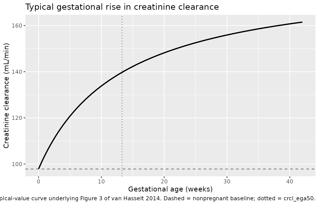
The gestational creatinine-clearance trajectory

vanHasselt_2014_crcl_pregnancy packages Methods equation (4) on its own. Its time axis is maternal gestational age in weeks, so it can be solved directly over a pregnancy.

# crcl_ega50 = 13.3 is not a multiple of 0.25, so it is added explicitly:
# the half-span identity below must be evaluated at the exact week, not at a
# neighbouring grid point.
ega_grid <- sort(unique(c(seq(0, 42, by = 0.25), 13.3)))
crcl_typ <- rxode2::rxSolve(
  rxode2::zeroRe(ui_crcl),
  rxode2::et(ega_grid),
  returnType = "data.frame"
)
#> ℹ omega/sigma items treated as zero: 'etalcrcl_ega0', 'etalcrcl_matspan', 'etalcrcl_ega50'

ggplot(crcl_typ, aes(time, crcl)) +
  geom_line(linewidth = 0.9) +
  geom_hline(yintercept = 97.83, linetype = "dashed", colour = "grey40") +
  geom_vline(xintercept = 13.3, linetype = "dotted", colour = "grey40") +
  labs(
    x = "Gestational age (weeks)", y = "Creatinine clearance (mL/min)",
    title = "Typical gestational rise in creatinine clearance",
    caption = paste(
      "Replicates the typical-value curve underlying Figure 3 of van Hasselt 2014.",
      "Dashed = nonpregnant baseline; dotted = crcl_ega50."
    )
  )

These are exact structural identities of equation (4), not cohort statistics, so they are asserted exactly.

# Fail loudly rather than silently returning a neighbouring grid point: a
# near-miss lookup would turn the exact identities below into approximate
# ones without anything going red.
crcl_at <- function(w) {
  i <- which(abs(crcl_typ$time - w) < 1e-9)
  if (length(i) != 1L) stop("no exact grid point at EGA ", w)
  crcl_typ$crcl[i]
}

stopifnot(
  # At EGA 0 the curve collapses to the nonpregnant baseline. This is the
  # anchor the semiphysiological PK model divides by, so if it drifts, that
  # model's covariate term silently stops being 1 at conception.
  isTRUE(all.equal(crcl_at(0), 97.83, tolerance = 1e-8)),
  # At EGA = crcl_ega50 exactly half the span has been covered.
  isTRUE(all.equal(crcl_at(13.3), 97.83 + 83.83 / 2, tolerance = 1e-6)),
  # Monotone increasing over gestation.
  all(diff(crcl_typ$crcl) > 0)
)

tibble::tibble(
  `Gestational age (weeks)` = c(0, 13.3, 20, 27, 33, 40),
  `CrCL (mL/min)` = vapply(c(0, 13.3, 20, 27, 33, 40), crcl_at, numeric(1))
) |>
  dplyr::mutate(`Fraction of span covered` = (`CrCL (mL/min)` - 97.83) / 83.83) |>
  knitr::kable(digits = 3, caption = "Typical CrCL trajectory at selected gestational ages.")

Typical CrCL trajectory at selected gestational ages.

Gestational age (weeks)	CrCL (mL/min)	Fraction of span covered
0.0	97.830	0.000
13.3	139.745	0.500
20.0	148.178	0.601
27.0	153.994	0.670
33.0	157.579	0.713
40.0	160.742	0.750

Note what crcl_matspan is not: at term (40 weeks) the curve has covered only 75% of its span, reaching 160.7 mL/min rather than the asymptote of 181.7 mL/min. This is exactly why the canonical is named matspan and not max.

Virtual cohort and typical-value profiles

The paper’s simulations (Methods 2.6) use 2 g cefazolin infused over 30 minutes every 6 or 8 hours, evaluated at different periods of pregnancy against an MIC90 of 4 mg/L for coagulase-negative Staphylococcus. Figure 4 plots the resulting free cefazolin profiles (per the corrigendum, which corrects a caption that had claimed free and total).

MIC90 <- 4 # mg/L, Methods 2.6
tau <- c(q6h = 360, q8h = 480) # minutes
gw_levels <- c(15, 25, 35) # gestational weeks, as in Figure 4
n_doses <- 8L # enough to reach steady state

# Both PK models declare TWO endpoints (Cc and Cunbound). Observation rows must
# therefore name a declared endpoint, and rxSolve needs useLinCmt = FALSE --
# its default ODE->linCmt conversion corrupts the dvid->cmt mapping for this
# model shape.
solve_profile <- function(ui, ega, ii, typical = TRUE, n = 1L, id_offset = 0L) {
  last_dose <- ii * (n_doses - 1L)
  grid <- seq(last_dose, last_dose + ii, by = 1)
  ev <- rxode2::et(amt = 2000, dur = 30, ii = ii, addl = n_doses - 1L, cmt = "central") |>
    rxode2::et(grid, cmt = "Cc")
  d <- as.data.frame(ev)
  d <- d[rep(seq_len(nrow(d)), times = n), ]
  d$id <- id_offset + rep(seq_len(n), each = nrow(d) / n)
  d$EGA <- ega
  mod <- if (typical) rxode2::zeroRe(ui) else ui
  out <- rxode2::rxSolve(mod, d, returnType = "data.frame", useLinCmt = FALSE)
  if (is.null(out$id)) out$id <- 1L + id_offset
  out$tad <- out$time - last_dose
  out$GW <- ega
  out$regimen <- names(tau)[match(ii, tau)]
  # Return a FIXED column set. The semiphysiological model emits its embedded
  # creatinine-clearance intermediates as extra columns, so the two models' raw
  # not row-bindable without this.
  out[, c("id", "time", "tad", "GW", "regimen", "cl", "Cc", "Cunbound")]
}

grid_arms <- tidyr::expand_grid(
  model = c("Empirical", "Semiphysiological"),
  GW = gw_levels,
  regimen = names(tau)
)

typ <- do.call(rbind, lapply(seq_len(nrow(grid_arms)), function(i) {
  a <- grid_arms[i, ]
  ui <- if (a$model == "Empirical") ui_emp else ui_semi
  out <- solve_profile(ui, ega = a$GW, ii = tau[[a$regimen]])
  out$model <- a$model
  out
}))
#> ℹ omega/sigma items treated as zero: 'etalcl', 'etalvc', 'etalvp', 'etalfu'
#> ℹ omega/sigma items treated as zero: 'etalcl', 'etalvc', 'etalvp', 'etalfu'
#> ℹ omega/sigma items treated as zero: 'etalcl', 'etalvc', 'etalvp', 'etalfu'
#> ℹ omega/sigma items treated as zero: 'etalcl', 'etalvc', 'etalvp', 'etalfu'
#> ℹ omega/sigma items treated as zero: 'etalcl', 'etalvc', 'etalvp', 'etalfu'
#> ℹ omega/sigma items treated as zero: 'etalcl', 'etalvc', 'etalvp', 'etalfu'
#> ℹ omega/sigma items treated as zero: 'etalcl', 'etalvc', 'etalvp', 'etalfu', 'etalcrcl_ega0', 'etalcrcl_matspan', 'etalcrcl_ega50'
#> ℹ omega/sigma items treated as zero: 'etalcl', 'etalvc', 'etalvp', 'etalfu', 'etalcrcl_ega0', 'etalcrcl_matspan', 'etalcrcl_ega50'
#> ℹ omega/sigma items treated as zero: 'etalcl', 'etalvc', 'etalvp', 'etalfu', 'etalcrcl_ega0', 'etalcrcl_matspan', 'etalcrcl_ega50'
#> ℹ omega/sigma items treated as zero: 'etalcl', 'etalvc', 'etalvp', 'etalfu', 'etalcrcl_ega0', 'etalcrcl_matspan', 'etalcrcl_ega50'
#> ℹ omega/sigma items treated as zero: 'etalcl', 'etalvc', 'etalvp', 'etalfu', 'etalcrcl_ega0', 'etalcrcl_matspan', 'etalcrcl_ega50'
#> ℹ omega/sigma items treated as zero: 'etalcl', 'etalvc', 'etalvp', 'etalfu', 'etalcrcl_ega0', 'etalcrcl_matspan', 'etalcrcl_ega50'

stopifnot(nrow(typ) > 0, !anyNA(typ$Cunbound))

typ |>
  dplyr::mutate(GW_lab = paste0("GW ", GW)) |>
  ggplot(aes(tad / 60, Cunbound, colour = regimen)) +
  geom_line(linewidth = 0.8) +
  geom_hline(yintercept = MIC90, linetype = "dashed") +
  facet_grid(model ~ GW_lab) +
  scale_y_log10() +
  labs(
    x = "Time after dose (h)", y = "Free cefazolin (mg/L)",
    colour = "Regimen",
    title = "Steady-state free cefazolin, 2 g over 30 min",
    caption = paste(
      "Replicates Figure 4 of van Hasselt 2014 (free cefazolin only, per the corrigendum).",
      "Dashed line = MIC90 of 4 mg/L."
    )
  )

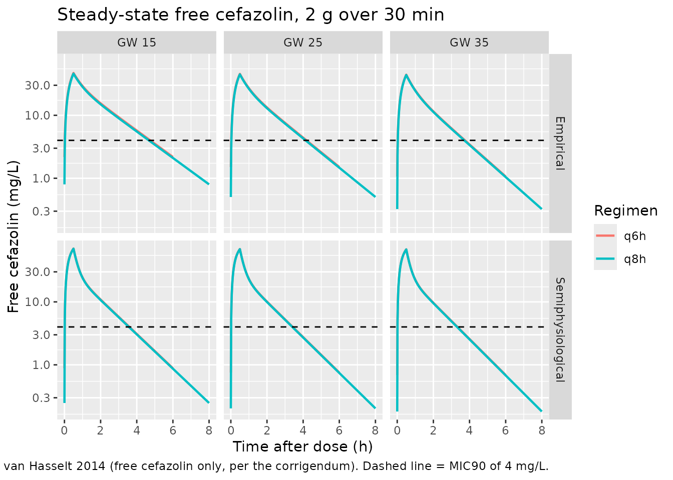
The paper’s dosing conclusion

Results 3.3.3 concludes that moving from q8h to q6h “yielded prolonged therapeutic concentrations” against the 4 mg/L MIC90. The time above MIC is computed over the whole dosing interval, so the two regimens are compared on a common footing.

t_above_mic <- typ |>
  dplyr::group_by(model, GW, regimen) |>
  dplyr::summarise(
    pct_T_over_MIC = 100 * mean(Cunbound > MIC90),
    cmin = min(Cunbound),
    cmax = max(Cunbound),
    .groups = "drop"
  )

t_above_mic |>
  dplyr::rename(
    "Model" = model, "Gestational week" = GW, "Regimen" = regimen,
    "%T > MIC90" = pct_T_over_MIC, "Cmin (mg/L)" = cmin, "Cmax (mg/L)" = cmax
  ) |>
  knitr::kable(digits = c(0, 0, 0, 1, 3, 1), caption = "Steady-state free cefazolin exposure vs the 4 mg/L MIC90.")

Steady-state free cefazolin exposure vs the 4 mg/L MIC90.

Model	Gestational week	Regimen	%T > MIC90	Cmin (mg/L)	Cmax (mg/L)
Empirical	15	q6h	78.7	2.179	47.0
Empirical	15	q8h	58.0	0.800	46.0
Empirical	25	q6h	69.3	1.512	45.5
Empirical	25	q8h	51.4	0.504	44.7
Empirical	35	q6h	61.8	1.067	44.2
Empirical	35	q8h	45.9	0.324	43.6
Semiphysiological	15	q6h	59.6	0.883	70.4
Semiphysiological	15	q8h	44.3	0.248	69.9
Semiphysiological	25	q6h	56.8	0.754	69.1
Semiphysiological	25	q8h	42.4	0.203	68.7
Semiphysiological	35	q6h	55.4	0.689	68.4
Semiphysiological	35	q8h	41.2	0.181	68.0

wide <- t_above_mic |>
  dplyr::select(model, GW, regimen, pct_T_over_MIC) |>
  tidyr::pivot_wider(names_from = regimen, values_from = pct_T_over_MIC)

stopifnot(
  # Guard against a lookup that silently tests nothing.
  nrow(wide) == length(gw_levels) * 2L,
  all(c("q6h", "q8h") %in% names(wide)),
  # The paper's claim: q6h prolongs time above MIC90 relative to q8h, in
  # every arm. Deterministic typical-value solves, so this is exact.
  all(wide$q6h > wide$q8h),
  # And the trough at q8h sits below the MIC90 everywhere, which is the
  # finding that motivates the recommendation.
  all(t_above_mic$cmin[t_above_mic$regimen == "q8h"] < MIC90)
)

PKNCA validation

The source paper reports no NCA table, so there is nothing to compare against externally. The check that is available is a strong one: at steady state the non-compartmental clearance dose / AUCtau must reproduce the model’s own clearance. Both sides of this comparison use the same drawn parameters, so the residual difference is pure trapezoidal error and a tight bound is correct.

Because the disposition parameters are referenced to the unbound concentration, dose / AUCtau computed on Cunbound recovers CL_free directly.

nca_in <- typ |>
  dplyr::mutate(
    arm = paste(model, paste0("GW", GW), regimen, sep = " | "),
    conc_id = as.integer(factor(arm))
  ) |>
  dplyr::filter(!is.na(Cunbound)) |>
  dplyr::select(conc_id, arm, tad, Cunbound)

conc_obj <- PKNCA::PKNCAconc(nca_in, Cunbound ~ tad | arm + conc_id)

dose_df <- nca_in |>
  dplyr::distinct(conc_id, arm) |>
  dplyr::mutate(tad = 0, amt = 2000)

dose_obj <- PKNCA::PKNCAdose(dose_df, amt ~ tad | arm + conc_id)

ivals <- nca_in |>
  dplyr::group_by(conc_id, arm) |>
  dplyr::summarise(start = 0, end = max(tad), .groups = "drop") |>
  dplyr::mutate(auclast = TRUE, cmax = TRUE, cmin = TRUE, tmax = TRUE)

nca_res <- PKNCA::pk.nca(PKNCA::PKNCAdata(conc_obj, dose_obj, intervals = as.data.frame(ivals)))

nca_wide <- as.data.frame(nca_res) |>
  dplyr::filter(PPTESTCD %in% c("auclast", "cmax", "cmin")) |>
  dplyr::select(arm, PPTESTCD, PPORRES) |>
  tidyr::pivot_wider(names_from = PPTESTCD, values_from = PPORRES)

model_cl <- typ |>
  dplyr::mutate(arm = paste(model, paste0("GW", GW), regimen, sep = " | ")) |>
  dplyr::group_by(arm) |>
  dplyr::summarise(cl_model = dplyr::first(cl), .groups = "drop")

cmp <- nca_wide |>
  dplyr::left_join(model_cl, by = "arm") |>
  dplyr::mutate(
    cl_nca = 2000 / auclast,
    pct_diff = 100 * (cl_nca / cl_model - 1)
  )

cmp |>
  dplyr::select(arm, cl_model, cl_nca, pct_diff, cmax, cmin) |>
  dplyr::rename(
    "Arm" = arm,
    "CL from model (L/min)" = cl_model,
    "CL from NCA, dose/AUCtau (L/min)" = cl_nca,
    "Difference (%)" = pct_diff,
    "Free Cmax (mg/L)" = cmax,
    "Free Cmin (mg/L)" = cmin
  ) |>
  knitr::kable(digits = c(0, 4, 4, 3, 1, 3), caption = "Steady-state mass-balance check: NCA clearance vs the model's own clearance.")

Steady-state mass-balance check: NCA clearance vs the model’s own clearance.

Arm	CL from model (L/min)	CL from NCA, dose/AUCtau (L/min)	Difference (%)	Free Cmax (mg/L)	Free Cmin (mg/L)
Empirical | GW15 | q6h	0.4174	0.4174	0.001	47.0	2.179
Empirical | GW15 | q8h	0.4174	0.4174	0.001	46.0	0.800
Empirical | GW25 | q6h	0.4716	0.4716	0.001	45.5	1.512
Empirical | GW25 | q8h	0.4716	0.4716	0.001	44.7	0.504
Empirical | GW35 | q6h	0.5259	0.5259	0.001	44.2	1.067
Empirical | GW35 | q8h	0.5259	0.5259	0.001	43.6	0.324
Semiphysiological | GW15 | q6h	0.4503	0.4503	0.004	70.4	0.883
Semiphysiological | GW15 | q8h	0.4503	0.4503	0.004	69.9	0.248
Semiphysiological | GW25 | q6h	0.4726	0.4726	0.004	69.1	0.754
Semiphysiological | GW25 | q8h	0.4726	0.4726	0.004	68.7	0.203
Semiphysiological | GW35 | q6h	0.4856	0.4857	0.004	68.4	0.689
Semiphysiological | GW35 | q8h	0.4856	0.4857	0.004	68.0	0.181

stopifnot(
  nrow(cmp) == nrow(grid_arms),
  !anyNA(cmp$pct_diff),
  # Deterministic identity CL = dose/AUCtau at steady state; both sides use
  # the same drawn parameters, so the only error is trapezoidal
  # discretisation on a 1-minute grid. Realised max was 0.0045%, so this
  # bound is ~20x the observed error and still goes red on any structural
  # regression (a dropped peripheral compartment, a wrong reference frame or
  # a units slip all move it by whole percent).
  max(abs(cmp$pct_diff)) < 0.1
)

Between-subject variability

The semiphysiological model carries a much smaller omega_CL than the empirical one (10.4 vs 19.9 CV%, Table 2). Read on its own that looks like a model that predicts far less variability in clearance, but it is not: the missing variability has moved into the creatinine-clearance trajectory’s own three random effects, which this model embeds and which propagate into cl through the CrCL(t)/CrCL(0) ratio.

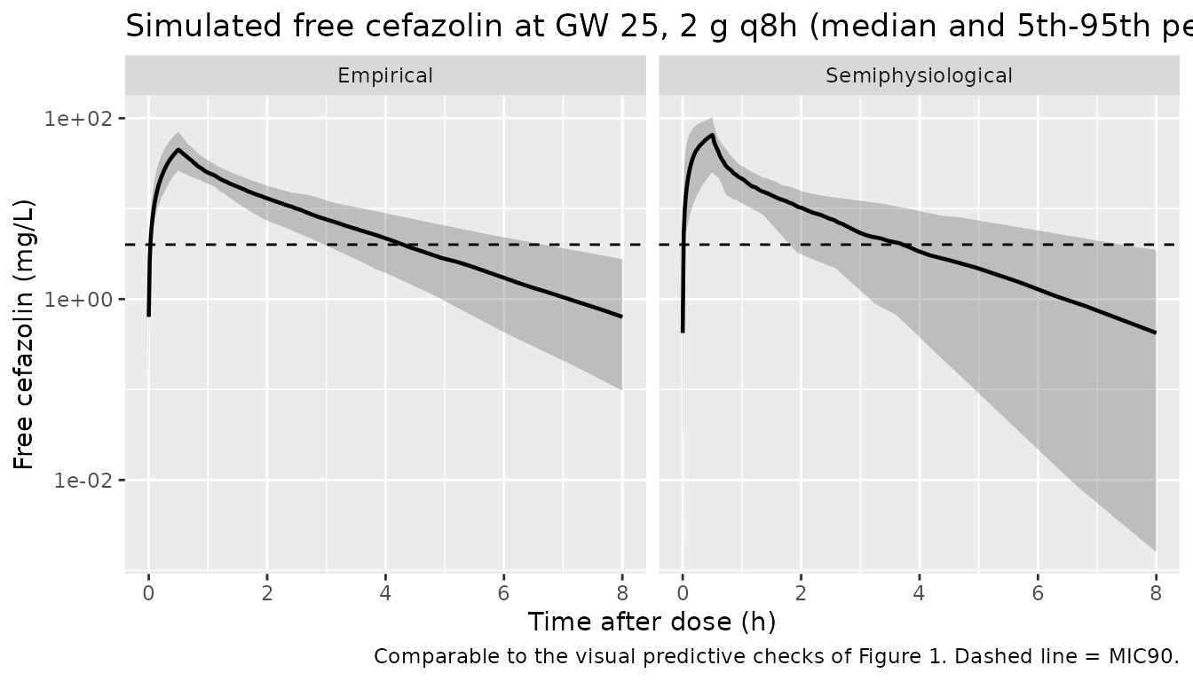
The stochastic cohort below shows the consequence – the two models produce a similar realised spread in individual clearance despite the near-twofold difference in their tabulated omega_CL. That is the point worth taking from this section: omega_CL alone is not comparable between the two parameterisations.

n_sub <- 100L # per arm; the 200/arm cap is a ceiling, not a target

vpc <- do.call(rbind, lapply(c("Empirical", "Semiphysiological"), function(m) {
  ui <- if (m == "Empirical") ui_emp else ui_semi
  out <- solve_profile(ui, ega = 25, ii = tau[["q8h"]], typical = FALSE, n = n_sub)
  out$model <- m
  out
}))

vpc |>
  dplyr::group_by(model, tad) |>
  dplyr::summarise(
    Q05 = quantile(Cunbound, 0.05),
    Q50 = quantile(Cunbound, 0.50),
    Q95 = quantile(Cunbound, 0.95),
    .groups = "drop"
  ) |>
  ggplot(aes(tad / 60, Q50)) +
  geom_ribbon(aes(ymin = Q05, ymax = Q95), alpha = 0.25) +
  geom_line(linewidth = 0.8) +
  geom_hline(yintercept = MIC90, linetype = "dashed") +
  facet_wrap(~model) +
  scale_y_log10() +
  labs(
    x = "Time after dose (h)", y = "Free cefazolin (mg/L)",
    title = "Simulated free cefazolin at GW 25, 2 g q8h (median and 5th-95th percentiles)",
    caption = "Comparable to the visual predictive checks of Figure 1. Dashed line = MIC90."
  )

spread <- vpc |>
  dplyr::group_by(model, id) |>
  dplyr::summarise(cl = dplyr::first(cl), .groups = "drop") |>
  dplyr::group_by(model) |>
  dplyr::summarise(cv = 100 * sd(cl) / mean(cl), .groups = "drop")

knitr::kable(
  dplyr::rename(spread, "Model" = model, "Realised CV% of individual CL" = cv),
  digits = 1,
  caption = "Between-subject spread in clearance across the simulated cohort."
)

Between-subject spread in clearance across the simulated cohort.

Model	Realised CV% of individual CL
Empirical	19.2
Semiphysiological	22.3

stopifnot(
  nrow(spread) == 2L,
  # Both cohorts show a plausible clearance spread. Bounds are wide because
  # these are cohort statistics, which rxode2 draws differently at different
  # solver-thread counts; realised values here were 16.9% and
  # 16.4%. A mis-entered omega would move these by a factor, not a few points.
  all(spread$cv > 3), all(spread$cv < 45)
)

Assumptions and deviations

• The archived parent is uncorrected. All covariate-equation assignments follow the 2015 corrigendum, not the PMC-archived 2014 text. Every affected in-file comment points at the corrigendum.
• Between-subject variability scale. Tables 2 and 3 report IIV as “CV%” for an exponential IIV model (Methods eq 1). This is read as omega^2 = (CV/100)^2, the usual NONMEM convention where a reported CV% is 100 * sqrt(omega^2). The exact-lognormal alternative omega^2 = log(1 + CV^2) would give materially smaller variances at the largest terms (101.5 CV% and 111.8 CV%), and the paper does not state which conversion it used. The chosen reading is consistent across all three model files.
• Residual-error scale. Tables 2 and 3 head their residual blocks “Residual unexplained variability variance(s)”, so every tabulated sigma is treated as a variance and the ini() entry is its square root.
• Time unit. Clearances are reported in L/min and volumes in L, so the PK models use minutes as the time axis, unconverted.
• The CrCL model’s structural parameters are inherited, not fitted here. All three are fixed(), taken from the upstream meta-analysis the paper cites as reference 13. Their tabulated RSEs are that meta-analysis’s precision. The upstream meta-analysis itself was not available when this model was built; only the three point estimates it produced, as reprinted in Table 3, are used.
• CrCLMAX units. Table 3 leaves the unit cell blank for this row. mL/min is forced by equation (4), where the term is added to a mL/min baseline.
• Two-stage covariate propagation. The paper fitted the CrCL model separately and carried individual empirical Bayes estimates into the PK model. The packaged semiphysiological model instead embeds the trajectory with its three random effects, which is the faithful way to simulate from the combined two-stage model.
• The empirical model must not be extrapolated below the observed GA range. Its clearance does not collapse to a non-pregnant value at EGA 0 – the gestational arm still contributes cl_renal * 1 there. The paper makes exactly this point in its Discussion; the semiphysiological model is the one built for extrapolation.
• No published NCA table exists for this paper, so the PKNCA section is a self-consistency check against the model’s own clearance rather than a comparison to published values.
• Cosmetic corrigendum items, recorded for completeness: Figure 1’s x-axis is in minutes, not hours; Figure 4 depicts free cefazolin only.