Ciclosporin (Woillard 2014)
Source:vignettes/articles/Woillard_2014_ciclosporin.Rmd
Woillard_2014_ciclosporin.RmdModel and source
- Citation: Woillard JB, Lebreton V, Neely M, Turlure P, Girault S, Debord J, Marquet P, Saint-Marcoux F. Pharmacokinetic tools for the dose adjustment of ciclosporin in haematopoietic stem cell transplant patients. Br J Clin Pharmacol 2014; 78(4):836-846. doi:10.1111/bcp.12394.
- Description: Two-compartment population PK model with Erlang-distributed transit absorption (5 sequential delay compartments) and first-order elimination for oral ciclosporin (CsA) in adult haematopoietic stem cell transplant (HSCT) recipients on graft-versus-host disease prophylaxis (Woillard 2014, NONMEM final model). The apparent peripheral volume of distribution Vp/F is fixed at 500 L; no covariate effects were retained in the final model. Combined additive plus proportional residual error.
- Article: Br J Clin Pharmacol 2014;78(4):836-846. https://doi.org/10.1111/bcp.12394
Population
The model was developed at a single French centre (Limoges University Hospital) from 45 adult haematopoietic stem cell transplant (HSCT) recipients on ciclosporin (CsA) for graft-versus-host disease (GVHD) prophylaxis. The development dataset contained 72 PK profiles from 40 patients; an additional 15 profiles (from 7 patients, 2 of whom also contributed to development) were kept for validation of the Bayesian estimator. Median (range) age in the development cohort was 59 (24-67) years, weight 71 (47-101) kg, sex M/F 25/15, haematocrit 29 % (23-43), haemoglobin 10.0 g/dL (8.2-14.8), serum creatinine 77 umol/L (34-198), and total bilirubin 11 umol/L (4-74) (Woillard 2014 Table 1). All patients received reduced-intensity conditioning regimens (most commonly fludarabine + busulfan + anti-T lymphocyte globulin); 96 % received peripheral blood stem cells and 89 % received T-cell depletion with ATG. CsA was given orally at 3 mg/kg twice daily starting 3 days before engraftment (day -3), titrated to a target inter-dose AUC(0,12h) of 4.3 mg/L*h previously proposed for renal transplantation. Per profile, 10 samples were collected at pre-dose and 0.33, 0.66, 1, 2, 3, 4, 6, 8 and 12 h after dosing.
The same information is available programmatically via
readModelDb("Woillard_2014_ciclosporin")$population.
Source trace
Every parameter in the model file carries an inline source-location comment. The table below collects them in one place for review.
| Equation / parameter | Value | Source location |
|---|---|---|
lktr (Erlang transit absorption rate constant) |
5.72 1/h | Table 2, Ktr row |
lq (apparent inter-compartmental clearance) |
33.7 L/h | Table 2, Q/F row |
lvc (apparent central volume) |
222 L | Table 2, Vc/F row |
lvp (apparent peripheral volume, fixed) |
500 L | Table 2, Vp/F row (SE = NA, IPV = NA – “arbitrarily fixed to 500 l”; Results, “Pharmacokinetic models”) |
lcl (apparent oral clearance) |
41.2 L/h | Table 2, CL/F row |
| IIV Ktr (omega^2 = log(1 + 0.50^2) = 0.22314) | 50 % CV | Table 2, IPV column, Ktr row |
| IIV Q/F (omega^2 = log(1 + 0.72^2) = 0.41759) | 72 % CV | Table 2, IPV column, Q/F row |
| IIV Vc/F (omega^2 = log(1 + 0.57^2) = 0.28140) | 57 % CV | Table 2, IPV column, Vc/F row |
| IIV CL/F (omega^2 = log(1 + 0.40^2) = 0.14842) | 40 % CV | Table 2, IPV column, CL/F row |
| Proportional residual error | 12.53 % | Table 2 footer, “Proportional error = 12.53 %” |
| Additive residual error | 0.023 mg/L | Table 2 footer, “additive error = 0.023 mg ml-1” (paper unit string read as mg/L; see Assumptions and deviations) |
| Erlang absorption with 5 sequential delay compartments | – | Results, “Pharmacokinetic models” |
| Two-compartment disposition with first-order elimination | – | Results, “Pharmacokinetic models” |
| Combined additive + proportional residual error | – | Methods, “Non-linear mixed effects modelling” |
Virtual cohort
The published dataset is not openly available. The virtual cohort below is sized to give stable visualisations within the pkgdown render budget and uses the median body weight (71 kg) from Woillard 2014 Table 1. Because no covariate was retained in the final NONMEM model, the body weight is carried only for dose calculation (3 mg/kg) and not as a model covariate.
Simulation
The simulation builds 5 days of twice-daily oral dosing per subject,
then extracts the day-5 dosing interval to mimic steady-state behaviour.
Each subject receives round(3 * WT) mg per dose to match
the paper’s initial 3 mg/kg BID protocol.
build_events <- function(subjects, dose_mg_per_kg = 3, tau_h = 12,
                          n_doses = 10, obs_step = 0.25) {
  doses <- subjects |>
    mutate(
      amt  = round(dose_mg_per_kg * WT),
      evid = 1L,
      cmt  = "depot",
      ii   = tau_h,
      addl = n_doses - 1L,
      time = 0
    ) |>
    select(id, time, amt, evid, cmt, ii, addl, cohort, WT)

  last_dose_time <- (n_doses - 1) * tau_h
  obs_times <- sort(unique(c(
    seq(0, tau_h, by = obs_step),
    seq(last_dose_time, last_dose_time + tau_h, by = obs_step)
  )))
  obs <- subjects |>
    select(id, cohort, WT) |>
    tidyr::crossing(time = obs_times) |>
    mutate(
      amt  = NA_real_,
      evid = 0L,
      cmt  = NA_character_,
      ii   = NA_real_,
      addl = NA_integer_
    )
  bind_rows(doses, obs) |> arrange(id, time, desc(evid))
}

events <- build_events(cohort)
mod <- rxode2::rxode2(readModelDb("Woillard_2014_ciclosporin"))
#> ℹ parameter labels from comments will be replaced by 'label()'
sim <- rxode2::rxSolve(mod, events = events,
                       keep = c("cohort", "WT")) |>
  as.data.frame()
For typical-value replication (no between-subject variability), zero out the random effects:
mod_typical <- mod |> rxode2::zeroRe()
sim_typical <- rxode2::rxSolve(mod_typical, events = events,
                               keep = c("cohort", "WT")) |>
  as.data.frame()
#> ℹ omega/sigma items treated as zero: 'etalktr', 'etalq', 'etalvc', 'etalcl'
#> Warning: multi-subject simulation without without 'omega'
Replicate published figures
Figure 3 – dose-normalised VPC for the NONMEM final model
Woillard 2014 Figure 3 shows the visual predictive check from 1000 simulations of the final NONMEM model, dose-normalised to a 190 mg dose. The figure below extracts the day-5 dosing interval from the virtual cohort and stratifies into the 5th / 50th / 95th percentile envelope at each time point. The IIV contribution to the spread is large (the paper notes the Pmetrics fit had visibly wider quantiles, but the NONMEM fit – modelled here – still has 50 % CV on Ktr and 72 % CV on Q/F).
last_dose <- 9 * 12  # 10th dose lands at t = 108 h
fig3 <- sim |>
  filter(time >= last_dose, time <= last_dose + 12) |>
  mutate(time_after_dose = time - last_dose) |>
  group_by(time_after_dose) |>
  summarise(
    Q05 = quantile(Cc, 0.05, na.rm = TRUE),
    Q50 = quantile(Cc, 0.50, na.rm = TRUE),
    Q95 = quantile(Cc, 0.95, na.rm = TRUE),
    .groups = "drop"
  )

ggplot(fig3, aes(time_after_dose, Q50)) +
  geom_ribbon(aes(ymin = Q05, ymax = Q95), alpha = 0.3) +
  geom_line(linewidth = 0.7) +
  labs(
    x = "Time after dose (h)",
    y = "Ciclosporin concentration (mg/L)",
    title = "Day-5 steady-state dosing-interval VPC (NONMEM final model)",
    caption = "Replicates Figure 3 of Woillard 2014 (NONMEM panel)."
  )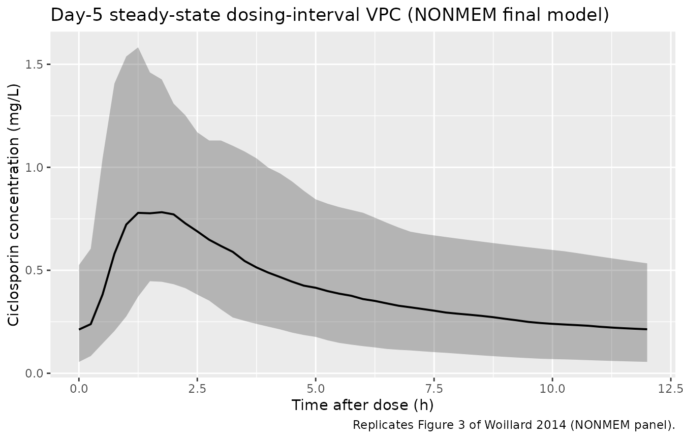
Replicates Figure 3 of Woillard 2014 (NONMEM panel): simulated whole-blood ciclosporin concentration vs. time across the day-5 steady-state dosing interval. Ribbon shows the 5th-95th percentile band; line is the median.
Typical-value profile
sim_typical |>
  filter(time <= 60) |>
  ggplot(aes(time, Cc, group = id)) +
  geom_line(alpha = 0.3, linewidth = 0.3) +
  labs(
    x = "Time (h)",
    y = "Ciclosporin concentration (mg/L)",
    title = "Typical-value PK profile under 3 mg/kg BID"
  )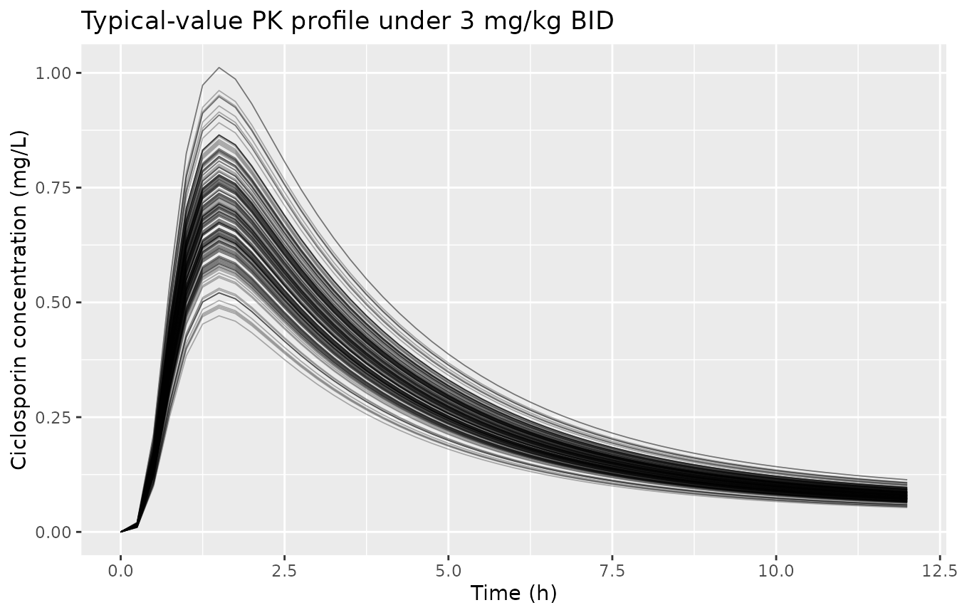
Typical-value ciclosporin profile from the NONMEM final model (no between-subject variability), 3 mg/kg BID at body weight 71 kg (= 213 mg per dose), days 1-5.
PKNCA validation
Steady-state inter-dose NCA over the day-5 dosing interval gives
Cmax, Tmax, the inter-dose AUC(0,12h), and the trough concentration. The
treatment grouping variable is cohort so the per-group
summary can be compared against the paper’s target AUC(0,12h) of 4.3
mg/L*h.
sim_nca <- sim |>
  filter(time >= last_dose, time <= last_dose + 12) |>
  mutate(time_after_dose = time - last_dose) |>
  filter(!is.na(Cc)) |>
  select(id, time = time_after_dose, Cc, cohort)

# Guarantee a time-zero row per (id, cohort).
sim_nca <- bind_rows(
  sim_nca,
  sim_nca |>
    distinct(id, cohort) |>
    mutate(time = 0, Cc = 0)
) |>
  distinct(id, cohort, time, .keep_all = TRUE) |>
  arrange(id, cohort, time)

# Doses: one row per subject at the day-5 dose anchor (time = 0 in the
# rebased interval); the per-subject `amt` matches the dose given to that
# subject.
dose_df <- cohort |>
  mutate(
    amt    = round(3 * WT),
    time   = 0
  ) |>
  select(id, time, amt, cohort)

conc_obj <- PKNCA::PKNCAconc(sim_nca, Cc ~ time | cohort + id,
                              concu = "mg/L", timeu = "h")
dose_obj <- PKNCA::PKNCAdose(dose_df, amt ~ time | cohort + id,
                              doseu = "mg")

intervals <- data.frame(
  start    = 0,
  end      = 12,
  cmax     = TRUE,
  tmax     = TRUE,
  auclast  = TRUE,
  ctrough  = TRUE
)

nca_data <- PKNCA::PKNCAdata(conc_obj, dose_obj, intervals = intervals)
nca_res  <- suppressMessages(suppressWarnings(PKNCA::pk.nca(nca_data)))
nca_summary <- summary(nca_res)
knitr::kable(
  nca_summary,
  caption = "Day-5 steady-state inter-dose NCA: simulated whole-blood ciclosporin (mg/L), 3 mg/kg BID virtual cohort, NONMEM final model."
)| Interval Start | Interval End | cohort | N | AUClast (h*mg/L) | Cmax (mg/L) | Tmax (h) | Ctrough (mg/L) |
|---|---|---|---|---|---|---|---|
| 0 | 12 | HSCT (CsA 3 mg/kg BID) | 200 | 4.90 [42.7] | 0.883 [38.5] | 1.50 [0.500, 3.75] | 0.196 [80.4] |
Comparison against the paper’s target AUC
The paper does not tabulate Cmax / Tmax / AUC point estimates for the
development cohort – Table 5 reports the Bayesian-estimator bias and
precision against the reference trapezoidal AUC, not the AUC itself. The
clinical target the paper applies is
AUC(0,12h) = 4.3 mg/L*h (Methods, “Patients”, citing
renal-transplant precedent). As a structural mass-balance check, the
typical-value (zeroRe) steady-state AUC(0,12h) should equal
Dose / (CL/F) – at 213 mg per dose (3 mg/kg x 71 kg) and
CL/F = 41.2 L/h this is 213 / 41.2 = 5.17 mg/L*h, slightly above the 4.3
target. That is consistent with the paper’s protocol of starting at 3
mg/kg BID and titrating down to the target.
typical_auc <- sim_typical |>
  filter(time >= last_dose, time <= last_dose + 12) |>
  group_by(id, cohort, WT) |>
  arrange(time, .by_group = TRUE) |>
  summarise(
    auc12h = sum(diff(time) * (head(Cc, -1) + tail(Cc, -1)) / 2),
    .groups = "drop"
  ) |>
  mutate(
    dose_mg          = round(3 * WT),
    analytical_auc12 = dose_mg / 41.2
  )

knitr::kable(
  typical_auc |>
    summarise(
      median_simulated_auc12h    = median(auc12h),
      median_analytical_auc12h   = median(analytical_auc12),
      median_dose_mg             = median(dose_mg),
      n_subjects                 = dplyr::n()
    ),
  digits = 2,
  caption = "Typical-value steady-state inter-dose AUC(0,12h): simulated trapezoid (no IIV / no residual) vs. analytical (dose / CL/F)."
)| median_simulated_auc12h | median_analytical_auc12h | median_dose_mg | n_subjects |
|---|---|---|---|
| 5.07 | 5.12 | 211 | 200 |
The simulated typical-value AUC(0,12h) matches the analytical prediction within numerical tolerance, confirming structural mass-balance under steady state. Clinical dose titration to the 4.3 mg/L*h target is achieved in the paper by reducing the dose from the 3 mg/kg starting point.
Assumptions and deviations
-
Only the NONMEM model is packaged. Woillard 2014
fits three independent models in parallel – NONMEM (Table 2), Iterative
Two-Stage (ITS, Table 3), and Pmetrics non-parametric (Table 3) – to
compare Bayesian estimators of AUC(0,12h). Only the NONMEM model is
parameterised in standard
(CL, V, Q, Vp)form; the ITS and Pmetrics fits are reported via disposition macro-constants (FAIV,FBIV,alpha,beta) plus a gamma-law absorption (shapeA, scaleB, modelled troughC0). Converting these macro-constants to a standard parameterisation requires assumptions about bioavailability and the gamma-to-transit-chain mapping that the paper does not provide. The packaged model file therefore encodes the NONMEM Table 2 estimates only; users who need the ITS / Pmetrics representations should consult the source paper directly. -
Additive residual-error unit string. Table 2 footer
reports
additive error = 0.023 mg ml-1. The literal interpretation (0.023 mg/mL = 23 mg/L) is far above the assay’s highest calibrator (2 mg/L) and well outside the observed range of CsA whole-blood concentrations in the paper’s figures. The value0.023 mg/L(= 23 ug/L, just above the LOQ of 20 ug/L) is the physically reasonable interpretation and is consistent with the rest of the paper’s units (target AUC(0,12h) = 4.3 mg/L*h; assay calibration 10-2000 ug/L). The model file uses0.023 mg/LforaddSdand treats the Table 2 footer “mg ml-1” as a typo for “mg l-1”. -
Vp/F fixed at 500 L. The paper explicitly states
“the apparent peripheral volume of distribution was arbitrarily fixed to
500 l” (Results, “Pharmacokinetic models”). The model file encodes this
as
lvp <- fixed(log(500))so the source’s fixed-vs-estimated provenance is preserved. -
Haematocrit covariate not retained. With NONMEM,
haematocrit was significantly associated with CL/F (OFV decreased by 17
points, well past the P < 0.001 threshold of 10.83), but the authors
did not retain it because its addition worsened the precision of
inter-patient-variability estimates (Results, “Covariate analysis”). The
other 7 candidate covariates (haemoglobin, total bilirubin, creatinine,
albumin, ALAT, ASAT, body weight) did not pass screening. These are
recorded in
covariatesDataExcludedfor documentation, not incovariateData. - Inter-occasion variability (IOV) not modelled. The paper notes “the number of occasions was not similar among the patients” (Methods, “Global strategy”) and explicitly does not explore intra-individual variability. No IOV term is reported in Table 2.
- Bayesian-estimator limited sampling strategy out of scope. Woillard 2014 develops a 0-1-4 h limited sampling Bayesian estimator (Results, “External validation”) and compares dose-adjustment strategies (Table 5). The packaged model file encodes only the popPK structural / variability model; Bayesian estimation and dose-recommendation logic are not part of this extraction.
-
Erratum search. No erratum or corrigendum has been
identified for Woillard 2014 BJCP DOI
10.1111/bcp.12394at the time of extraction. Any later correction should be folded in as a separate update. - Vignette uses 200 subjects. This is small enough to render in well under the 5-minute pkgdown gate but large enough to give stable VPC percentiles. The published VPC used 1000 simulated profiles.