Atenolol + metoprolol absorption in malnourished rats (Kir 2025)
Source:vignettes/articles/Kir_2025_atenolol_metoprolol_malnutrition.Rmd
Kir_2025_atenolol_metoprolol_malnutrition.RmdModel and source
This paper contributes two model files – one per drug – because the two minimal PBPK (mPBPK) structures differ mechanistically, not just numerically: atenolol is eliminated by the kidney with permeability-limited distribution, metoprolol by the liver with perfusion-limited distribution and a structural first-pass effect.
mod_atn <- readModelDb("Kir_2025_atenolol_rat_pbpk")
mod_met <- readModelDb("Kir_2025_metoprolol_rat_pbpk")

ui_atn <- rxode2::rxode(mod_atn)
#> ℹ parameter labels from comments will be replaced by 'label()'
ui_met <- rxode2::rxode(mod_met)
#> ℹ parameter labels from comments will be replaced by 'label()'- Citation: Kir F, Sahin S, Jusko WJ. Minimal Physiologically-Based Pharmacokinetic Modeling of Atenolol and Metoprolol Absorption in Malnourished Rats. Eur J Drug Metab Pharmacokinet. 2025;50(3):251-263. doi:10.1007/s13318-025-00943-6. PMCID PMC12081501. Population parameter estimates: Table 2 (Monolix). Naive-pooled (ADAPT 5) estimates for the same model: Supplementary Table S3. Rat physiology (tissue volumes and blood flows): Supplementary Table S2. Model equations: Article Equations 1-5 (ATN), 9 (tissue-volume closure), 10 (permeability-limited fd constraint) and 12 (blood-to-plasma ratio). ODEs, fixed system constants and the absorption-window logic were taken from the author-deposited Monolix (MLXTRAN) and ADAPT-5 source listings in the Supplementary Materials, which agree with each other exactly.
- Article: https://doi.org/10.1007/s13318-025-00943-6
- Supplement (parameter tables S1-S4 and the author-deposited Monolix / ADAPT-5 source listings): https://doi.org/10.1007/s13318-025-00943-6
Atenolol model. Preclinical (rat, Sprague-Dawley). mPBPK (minimal physiologically-based, Monolix 2023R1 population fit). Atenolol (ATN) oral absorption in non-malnourished (control) and malnourished rats. Four mass-balance states: a well-mixed blood pool, two lumped tissue groups (Tissue 1 = rapidly perfused liver + lung, high Kp; Tissue 2 = slowly perfused remainder) and the kidney, which is the eliminating organ (ATN is hydrophilic, logP 0.16, and is cleared almost entirely renally). Distribution is PERMEABILITY-limited: the fraction of cardiac output actually equilibrating with each tissue group is small and estimated (fd1 = fd2 = 0.134, so only ~27% of cardiac output is distributive), which is what encodes atenolol’s BCS Class III low permeability. Oral input is NOT first-order: the paper’s point-area deconvolution showed a near-constant absorption rate over successive time windows, so absorption is modelled as two (control) or three (malnourished) SEQUENTIAL ZERO-ORDER processes with author-fixed window boundaries (0-120, 120-300, and 300-420 min). Malnutrition acts on ABSORPTION only – disposition (fd1, Kp1, CL) is shared across groups, and the malnourished group gains a third absorption phase (k03 = 1.16 mg/min/kg, fixed to 0 in controls by goodness of fit) that raises apparent bioavailability from 0.43 to 0.67. Blood-to-plasma ratio differs by group (1.000 vs 1.014) because malnutrition changes haematocrit and albumin binding. The model as shipped simulates the ORAL arms; the literature IV reference profile is reproduced by setting k01/k02/k03 to 0 and giving a bolus into a_blood (see the vignette). IIV is on clearance only. NOTE: the absorption-rate scale in Tables 2/3 required reconciliation against the deposited Monolix code – see the vignette Errata.
Metoprolol model. Preclinical (rat, Sprague-Dawley). mPBPK (minimal physiologically-based, Monolix 2023R1 population fit). Metoprolol (MET) oral absorption in non-malnourished (control) and malnourished rats. Sister model to modellib(‘Kir_2025_atenolol_rat_pbpk’) from the same paper, and deliberately contrasted with it: metoprolol is lipophilic (logP 1.76, BCS Class I) and hepatically extracted, so the eliminating organ is the LIVER rather than the kidney, distribution is PERFUSION-limited (fd1 + fd2 = 1 exactly, versus 0.268 for atenolol), and Tissue 1 is kidney + lung rather than liver + lung. Four mass-balance states: a well-mixed blood pool, two lumped tissue groups (Tissue 1 rapidly perfused, high Kp; Tissue 2 slowly perfused remainder) and the liver. Crucially the oral zero-order input is delivered INTO THE LIVER, so hepatic first-pass extraction is structural rather than a fitted F – roughly 50% of an oral dose is lost on first pass. Absorption is two SEQUENTIAL ZERO-ORDER processes with author-fixed windows (0-60 min, then 60-135 min in controls and 60-110 min in the malnourished group). Malnutrition raises both absorption rates and shortens the second window, taking apparent bioavailability from 0.42 to 0.84. The oral arms also carry an estimated FRACTION of the IV intrinsic clearance (fr = 0.336 control, 0.256 malnourished) rather than the full CLint, which is how the published fit reconciles the oral decline phases with the literature IV data. Blood-to-plasma ratio differs by group (1.508 vs 1.607). The model as shipped simulates the ORAL arms; the literature IV reference profile is reproduced by setting k01/k02 to 0, fr to 1 and bpr to 1.70, and giving a bolus into a_blood (see the vignette). IIV is on intrinsic clearance only. NOTE: the absorption-rate scale in Tables 2/3 required reconciliation against the deposited Monolix code – see the vignette Errata.
Population
Eight male Sprague-Dawley rats per drug (n = 4 control, n = 4 malnourished) were studied. Malnutrition was induced by feeding a 5% protein isocaloric diet for 17-20 days; controls received a 20% protein isocaloric diet. Table 1 of the paper confirms that the intervention worked: body weight fell from 300 to 216 g (atenolol cohort) and 302 to 233 g (metoprolol cohort), serum albumin from 4.40 to 3.75 and 4.68 to 4.15 g/dL, and total cholesterol from 78.4 to 50.3 and 66.5 to 49.5 mg/dL.
Rats were fasted overnight and given a single oral dose by feeding tube: 250 mg/kg atenolol as an aqueous suspension, or 400 mg/kg metoprolol tartrate (equal to 312 mg/kg metoprolol base) in solution. These are deliberately high doses chosen from pilot studies so that the absorption phase is resolvable.
Critically, no intravenous dose was given in this study. The IV reference profiles that identify disposition were digitised from the literature (atenolol 1 mg/kg; metoprolol 0.5, 1 and 2 mg/kg, shown to be dose-linear), and the per-timepoint standard deviations were digitised and treated as additional rats so that the pooled fit had IV replicates.
The same information is available programmatically via each model’s
population metadata:
str(ui_atn$population, max.level = 1)
#> List of 10
#>  $ species       : chr "rat (Sprague-Dawley)"
#>  $ n_subjects    : int 8
#>  $ n_studies     : int 2
#>  $ age_range     : chr NA
#>  $ weight_range  : chr "216 (SD 14.99) g malnourished to 300 (SD 18.27) g control"
#>  $ sex_female_pct: num 0
#>  $ disease_state : chr "Experimental protein-calorie malnutrition (5% protein isocaloric diet, 17-20 days) vs control (20% protein isocaloric diet)"
#>  $ dose_range    : chr "250 mg/kg single oral dose (suspension, feeding tube); literature IV reference 1 mg/kg"
#>  $ regions       : chr "Turkey (Kobay Experimental Animals Laboratory, Ankara)"
#>  $ notes         : chr "n = 4 control + 4 malnourished male Sprague-Dawley rats (Methods 2.2.1); the oral arms are the only rats actual"| __truncated__
Source trace
The per-parameter origin is recorded as an in-file comment next to
each ini() entry in
inst/modeldb/specificDrugs/Kir_2025_atenolol_rat_pbpk.R and
inst/modeldb/specificDrugs/Kir_2025_metoprolol_rat_pbpk.R.
The table below collects them for review.
| Equation / parameter | Value (ATN / MET) | Source location |
|---|---|---|
| Blood-compartment ODE | n/a | Equation 1 (ATN) / Equation 6 (MET); deposited Monolix
ddt_B, ADAPT XP(1)
|
| Tissue 1 and Tissue 2 ODEs | n/a | Equations 2-3 (ATN) / 7 (MET); deposited ddt_T1,
ddt_T2
|
| Eliminating-organ ODE | n/a | Equation 4 (ATN, kidney) / Equation 8 (MET, liver); deposited
ddt_K / ddt_L
|
| Tissue-volume closure | Body weight = Vb + V1 + V2 + V3 | Equation 9 |
| Distribution constraint | fd1 + fd2 <= 1 (ATN) / fd1 + fd2 = 1 (MET) | Equation 10 (ATN) / Equation 11 (MET) |
| Blood-to-plasma ratio | rho = (HCT - 1 + Rb) / (HCT * fu) | Equation 12 |
v_blood |
58.82 mL/kg | Supp Table S2; deposited Vb
|
v_rapidly_perfused |
37.08 / 9.43 mL/kg | Supp Table S2 (ATN liver+lung; MET kidney+lung); deposited
V1
|
v_slowly_perfused |
897.94 mL/kg | Equation 9 closure; deposited V2
|
v_kidney / v_liver
|
6.16 / 33.81 mL/kg | Supp Table S2; deposited Vkid /
Vliver
|
q_co |
179.91 mL/min/kg | Supp Table S2; deposited Qco
|
q_kidney / q_liver
|
29.00 / 75.34 mL/min/kg | Supp Table S2; deposited Qkid /
Qliver
|
kp_kidney / kp_liver
|
3.0 / 62.25 | Methods 2.2.2 / 2.2.3 (GastroPlus 9.9 predictions) |
bpr_control |
1.000 / 1.508 | Methods 2.2.3; deposited Rb_H
|
bpr_malnourished |
1.014 / 1.607 | Methods 2.2.3 |
fd_rapidly_perfused |
0.134 / 0.464 | Table 2 / Table 3 |
kp_rapidly_perfused |
1.43 / 4.033 | Table 2 / Table 3 |
lcl / lclint
|
log(16.04) / log(148.63) | Table 2 CL / Table 3 CLint (deposited code carries the unrounded 148.63) |
fr_control, fr_malnourished
|
n/a / 0.336, 0.256 | Table 3 |
k01, k02, k03 (per
group) |
Table 2 / Table 3 | Table 2 (ATN, 3 phases) / Table 3 (MET, 2 phases) |
| Absorption windows | 120, 300, 360/420 min / 60, 135 or 110 min | Results 3.1 (all fixed, not estimated) |
etalcl / etalclint
|
0.124^2 / 0.258^2 | Table 2 / Table 3 “Standard deviation of the random effects” |
propSd (ATN) / addSd (MET) |
0.256, 0.234 / 1.76, 2.54 | Table 2 b C, b M / Table 3 a C, a M |
dose_po |
250 / 312.3274 mg/kg | Methods 2.2.1; deposited multipliers 250000 and 312327.4 ug/kg |
Structural checks against the published equations
Two of the paper’s equations are closed-form identities that the packaged fixed constants must satisfy exactly. These are cheap, sharp regression guards: they fail loudly if any physiological constant is mistranscribed.
# Equation 9: Body weight = Vb + V1 + V2 + V3. All volumes are mL/kg, so the
# sum must be exactly 1000 mL/kg for both drugs.
theta <- function(ui, nm) ui$theta[[nm]]

vol_atn <- c(theta(ui_atn, "v_blood"), theta(ui_atn, "v_rapidly_perfused"),
             theta(ui_atn, "v_slowly_perfused"), theta(ui_atn, "v_kidney"))
vol_met <- c(theta(ui_met, "v_blood"), theta(ui_met, "v_rapidly_perfused"),
             theta(ui_met, "v_slowly_perfused"), theta(ui_met, "v_liver"))

stopifnot(isTRUE(all.equal(sum(vol_atn), 1000)), isTRUE(all.equal(sum(vol_met), 1000)))
c(atenolol = sum(vol_atn), metoprolol = sum(vol_met))
#>   atenolol metoprolol
#>       1000       1000
# Tissue 1 is a LUMP of named organs from Supplementary Table S2:
#   atenolol   -> liver + lung  (kidney is the separate eliminating organ)
#   metoprolol -> kidney + lung (liver is the separate eliminating organ)
v_lung <- 3.27; v_liver_s2 <- 33.81; v_kidney_s2 <- 6.16   # Supp Table S2
stopifnot(
  isTRUE(all.equal(theta(ui_atn, "v_rapidly_perfused"), v_liver_s2 + v_lung)),
  isTRUE(all.equal(theta(ui_met, "v_rapidly_perfused"), v_kidney_s2 + v_lung))
)
# Equation 12 rearranged: Rb = 1 - HCT + rho * HCT * fu.
# HCT 47.5% control / 45.5% malnourished (Methods 2.2.3, reference 30).
# fu: ATN 0.970 -> 1.00, MET 0.805 -> 0.908 (rescaled by the albumin ratio).
# rho is fixed at 2.57 for metoprolol; for atenolol it is back-calculated from
# the control Rb of 1.000, then reused for the malnourished group.
rb <- function(rho, hct, fu) 1 - hct + rho * hct * fu

rho_atn <- (0.475 - 1 + 1.000) / (0.475 * 0.970)   # solve Equation 12 for rho
rho_met <- 2.57                                     # Methods 2.2.3, fixed

eq12 <- tibble::tibble(
  drug  = c("atenolol", "atenolol", "metoprolol", "metoprolol"),
  group = c("control", "malnourished", "control", "malnourished"),
  equation_12 = c(rb(rho_atn, 0.475, 0.970), rb(rho_atn, 0.455, 1.000),
                  rb(rho_met, 0.475, 0.805), rb(rho_met, 0.455, 0.908)),
  packaged = c(theta(ui_atn, "bpr_control"), theta(ui_atn, "bpr_malnourished"),
               theta(ui_met, "bpr_control"), theta(ui_met, "bpr_malnourished"))
)

stopifnot(all(abs(eq12$equation_12 - eq12$packaged) < 5e-4))

eq12 |>
  dplyr::mutate(dplyr::across(c(equation_12, packaged), \(x) round(x, 4))) |>
  dplyr::rename("Drug" = drug, "Group" = group,
                "Equation 12" = equation_12, "Packaged value" = packaged) |>
knitr::kable(caption = "Equation 12 reproduces every packaged blood-to-plasma ratio.")| Drug | Group | Equation 12 | Packaged value |
|---|---|---|---|
| atenolol | control | 1.0000 | 1.000 |
| atenolol | malnourished | 1.0141 | 1.014 |
| metoprolol | control | 1.5077 | 1.508 |
| metoprolol | malnourished | 1.6068 | 1.607 |
Virtual cohort
The original per-rat data are not distributed, so the simulations below use the model’s own typical-value predictions (which is what Figures 4 and 5 of the paper plot) plus a small stochastic cohort for a visual predictive check.
Note that the oral arms carry no dosing event. The
published model drives absorption entirely from elapsed time via the
sequential zero-order windows, so the event table holds observation rows
only; the dose enters through the dose_po parameter.
Observation rows point at the a_blood ODE state, and rxode2
returns the algebraic observable Cc alongside it.
set.seed(20250409)

n_per_arm <- 50L   # well under the 200/arm cap

# Observation-only event table for one arm of the oral study.
make_oral_arm <- function(n, mal, tmax, by = 5, id_offset = 0L) {
  tidyr::expand_grid(
    id   = id_offset + seq_len(n),
    time = seq(0, tmax, by = by)
  ) |>
    dplyr::mutate(
      amt         = NA_real_,
      evid        = 0L,
      cmt         = "a_blood",
      MAL_NOURISH = mal
    )
}

arms <- tibble::tribble(
  ~drug,        ~group,         ~mal, ~tmax_obs,
  "atenolol",   "control",         0,       480,
  "atenolol",   "malnourished",    1,       480,
  "metoprolol", "control",         0,       420,
  "metoprolol", "malnourished",    1,       420
) |>
  dplyr::mutate(treatment = paste(drug, group, sep = " / "))

events <- dplyr::bind_rows(
  lapply(seq_len(nrow(arms)), function(i) {
    make_oral_arm(n_per_arm, arms$mal[i], arms$tmax_obs[i],
                  id_offset = (i - 1L) * n_per_arm) |>
      dplyr::mutate(drug = arms$drug[i], group = arms$group[i],
                    treatment = arms$treatment[i])
  })
)

# Disjoint IDs across arms are mandatory -- duplicate IDs silently merge.
stopifnot(!anyDuplicated(unique(events[, c("id", "time", "evid")])))
Simulation
Figures 4 and 5 of the paper are population fits – single lines through the observed points – so the replication below zeroes the random effects.
solve_typical <- function(ui, ev) {
  out <- as.data.frame(
    rxode2::rxSolve(rxode2::zeroRe(ui), ev,
                    keep = c("drug", "group", "treatment"))
  )
  if (is.null(out$id)) out$id <- 1L
  out
}

sim_typ <- dplyr::bind_rows(
  solve_typical(ui_atn, dplyr::filter(events, drug == "atenolol",   id <= n_per_arm * 2)),
  solve_typical(ui_met, dplyr::filter(events, drug == "metoprolol", id >  n_per_arm * 2))
)
#> Warning: No sigma parameters in the model
#> ℹ omega/sigma items treated as zero: 'etalcl'
#> Warning: multi-subject simulation without without 'omega'
#> Warning: No sigma parameters in the model
#> ℹ omega/sigma items treated as zero: 'etalclint'
#> Warning: multi-subject simulation without without 'omega'

# Every arm must have produced finite, non-negative concentrations.
stopifnot(all(is.finite(sim_typ$Cc)), all(sim_typ$Cc >= -1e-8),
          dplyr::n_distinct(sim_typ$treatment) == 4L)
sim_vpc <- dplyr::bind_rows(
  as.data.frame(rxode2::rxSolve(
    ui_atn, dplyr::filter(events, drug == "atenolol", id <= n_per_arm * 2),
    keep = c("drug", "group", "treatment"))),
  as.data.frame(rxode2::rxSolve(
    ui_met, dplyr::filter(events, drug == "metoprolol", id > n_per_arm * 2),
    keep = c("drug", "group", "treatment")))
)

# rxSolve silently drops subjects on failure -- assert the count survived.
stopifnot(dplyr::n_distinct(sim_vpc$id) == n_per_arm * 4L)
Replicate published figures
# Replicates the "Control" and "Malnourished" panels of Figure 4 (atenolol)
# and Figure 5 (metoprolol) of Kir 2025: population fits of plasma
# concentration versus time.
obs_cmax <- tibble::tribble(
  ~treatment,                     ~cmax_obs, ~tmax_obs,
  "atenolol / control",               24.02,       240,
  "atenolol / malnourished",          23.46,       240,
  "metoprolol / control",             14.34,       120,
  "metoprolol / malnourished",        23.04,      93.8
)

sim_typ |>
  dplyr::filter(id %in% c(1L, n_per_arm + 1L, n_per_arm * 2 + 1L, n_per_arm * 3 + 1L)) |>
  ggplot(aes(time, Cc)) +
  geom_line(linewidth = 0.8) +
  geom_point(data = obs_cmax, aes(x = tmax_obs, y = cmax_obs),
             colour = "firebrick", size = 2.5, inherit.aes = FALSE) +
  facet_wrap(~treatment, scales = "free_x") +
  labs(x = "Time (min)", y = "Plasma concentration (ug/mL)",
       title = "Figures 4 and 5 -- population fits, oral arms",
       caption = paste("Lines replicate the Control and Malnourished panels of",
                       "Figure 4 (atenolol) and Figure 5 (metoprolol) of Kir 2025.",
                       "Red points are the observed group-mean Cmax / Tmax",
                       "from Supplementary Table S1."))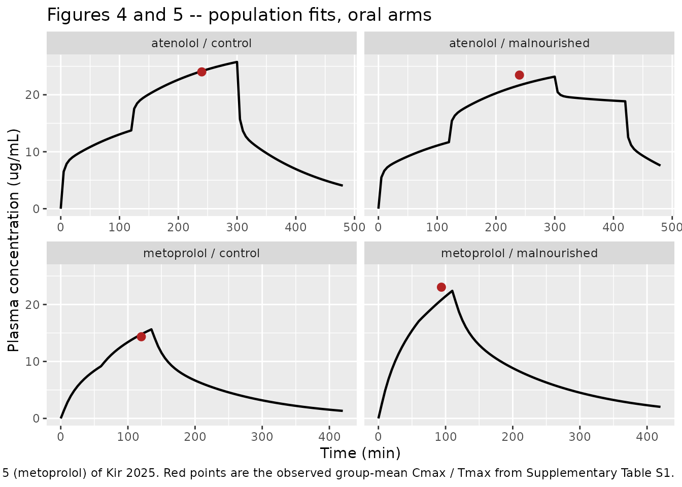
The sharp cusps are real features of the published model, not solver artefacts: absorption stops abruptly at the end of the last zero-order window (300 min for atenolol controls, 420 min for malnourished atenolol, 135 and 110 min for the metoprolol groups), and the profile turns over immediately.
sim_vpc |>
  dplyr::group_by(treatment, time) |>
  dplyr::summarise(
    Q05 = quantile(Cc, 0.05, na.rm = TRUE),
    Q50 = quantile(Cc, 0.50, na.rm = TRUE),
    Q95 = quantile(Cc, 0.95, na.rm = TRUE),
    .groups = "drop"
  ) |>
  ggplot(aes(time, Q50)) +
  geom_ribbon(aes(ymin = Q05, ymax = Q95), alpha = 0.25) +
  geom_line() +
  facet_wrap(~treatment, scales = "free_x") +
  labs(x = "Time (min)", y = "Plasma concentration (ug/mL)",
       title = "Visual predictive check (5th-95th percentile)",
       caption = paste("Between-subject variability is on clearance only",
                       "(omega 0.124 for atenolol, 0.258 for metoprolol),",
                       "so the ribbon is narrow during absorption and widens",
                       "through the elimination phase."))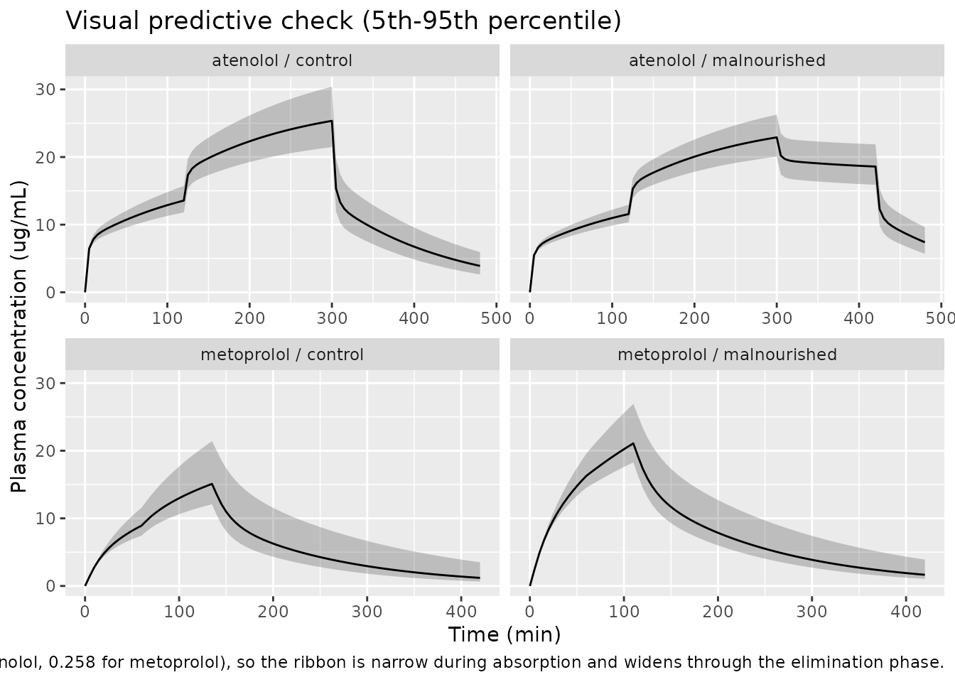
Reproducing the literature IV reference profiles
The disposition block is identified entirely by the digitised
literature IV data, so simulating the IV arm is an independent check on
fd1, Kp1, CL and the organ flows
– none of which the oral figures constrain directly. The IV arm is
obtained by zeroing the absorption rates and giving a bolus into
a_blood; for metoprolol the IV reference additionally used
the full intrinsic clearance (fr = 1) and the racemate
blood-to-plasma ratio of 1.70.
iv_events <- function(dose_ug_kg, tmax) {
  dplyr::bind_rows(
    data.frame(id = 1L, time = 0, amt = dose_ug_kg, evid = 1L, cmt = "a_blood"),
    data.frame(id = 1L, time = seq(0, tmax, by = 1), amt = NA_real_,
               evid = 0L, cmt = "a_blood")
  ) |>
    dplyr::mutate(MAL_NOURISH = 0) |>
    dplyr::arrange(time, dplyr::desc(evid))
}

ui_atn_iv <- rxode2::ini(ui_atn, k01_control = 0, k02_control = 0, k03_control = 0)
#> ℹ change initial estimate of `k01_control` to `0`
#> ℹ change initial estimate of `k02_control` to `0`
#> ℹ change initial estimate of `k03_control` to `0`
ui_met_iv <- rxode2::ini(ui_met, k01_control = 0, k02_control = 0,
                         fr_control = 1, bpr_control = 1.70)
#> ℹ change initial estimate of `k01_control` to `0`
#> ℹ change initial estimate of `k02_control` to `0`
#> ℹ change initial estimate of `fr_control` to `1`
#> ℹ change initial estimate of `bpr_control` to `1.7`

sim_iv <- dplyr::bind_rows(
  as.data.frame(rxode2::rxSolve(rxode2::zeroRe(ui_atn_iv), iv_events(1000, 480))) |>
    dplyr::mutate(drug = "atenolol 1 mg/kg IV"),
  as.data.frame(rxode2::rxSolve(rxode2::zeroRe(ui_met_iv), iv_events(1000, 180))) |>
    dplyr::mutate(drug = "metoprolol 1 mg/kg IV")
)
#> Warning: No sigma parameters in the model
#> ℹ omega/sigma items treated as zero: 'etalcl'
#> Warning: No sigma parameters in the model
#> ℹ omega/sigma items treated as zero: 'etalclint'

sim_iv |>
  dplyr::filter(Cc > 1e-4) |>
  ggplot(aes(time, Cc)) +
  geom_line(linewidth = 0.8) +
  facet_wrap(~drug, scales = "free") +
  scale_y_log10() +
  labs(x = "Time (min)", y = "Plasma concentration (ug/mL)",
       title = "Figures 4 and 5 -- IV reference panels",
       caption = paste("Replicates the IV panel of Figure 4 (atenolol,",
                       "1 mg/kg) and Figure 5 (metoprolol, 1 mg/kg) of",
                       "Kir 2025. Both are biexponential, as the paper",
                       "describes."))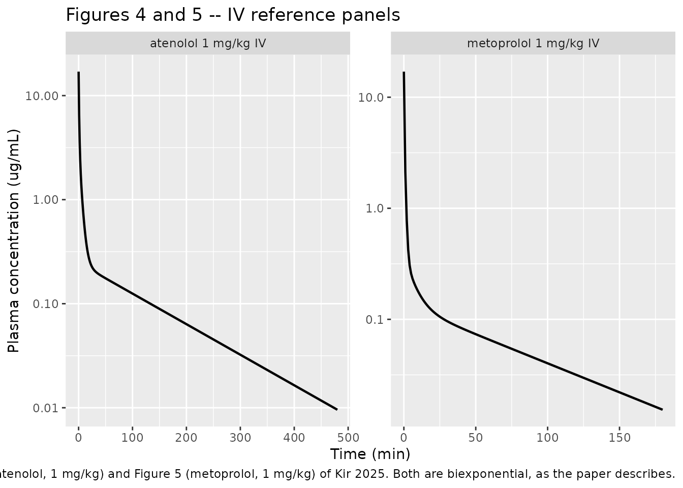
Both IV profiles are biexponential over roughly two to three log units, which is what the paper reports (“ATN exhibited a rapid initial decline phase followed by a long linear terminal phase”; “MET also exhibited apparent IV biexponential disposition kinetics”).
PKNCA validation
# NCA runs on the typical-value profile over a window long enough for the
# terminal phase to resolve. Only !is.na(Cc) is filtered -- adding time > 0 or
# Cc > 0 would drop the time-zero anchor PKNCA needs for AUC0-*.
nca_events <- dplyr::bind_rows(
  lapply(seq_len(nrow(arms)), function(i) {
    data.frame(id = i, time = seq(0, 1440, by = 2), amt = NA_real_,
               evid = 0L, cmt = "a_blood", MAL_NOURISH = arms$mal[i],
               drug = arms$drug[i], treatment = arms$treatment[i])
  })
)

sim_nca_raw <- dplyr::bind_rows(
  solve_typical(ui_atn, dplyr::filter(nca_events, drug == "atenolol") |>
                  dplyr::mutate(group = "x")),
  solve_typical(ui_met, dplyr::filter(nca_events, drug == "metoprolol") |>
                  dplyr::mutate(group = "x"))
)
#> Warning: No sigma parameters in the model
#> ℹ omega/sigma items treated as zero: 'etalcl'
#> Warning: multi-subject simulation without without 'omega'
#> Warning: No sigma parameters in the model
#> ℹ omega/sigma items treated as zero: 'etalclint'
#> Warning: multi-subject simulation without without 'omega'

sim_nca <- sim_nca_raw |>
  dplyr::filter(!is.na(Cc)) |>
  dplyr::mutate(Cc = pmax(Cc, 0)) |>       # guard the far tail against solver noise
  dplyr::select(id, time, Cc, treatment)

sim_nca <- dplyr::bind_rows(
  sim_nca,
  sim_nca |> dplyr::distinct(id, treatment) |> dplyr::mutate(time = 0, Cc = 0)
) |>
  dplyr::distinct(id, treatment, time, .keep_all = TRUE) |>
  dplyr::arrange(id, treatment, time)

stopifnot(nrow(sim_nca) > 0, all(sim_nca$Cc >= 0))

conc_obj <- PKNCA::PKNCAconc(sim_nca, Cc ~ time | treatment + id)

# One dose row per arm. There is no evid == 1 record in the oral event table
# (absorption is time-driven), so the dose amount comes from dose_po.
dose_df <- arms |>
  dplyr::mutate(
    id   = dplyr::row_number(),
    time = 0,
    amt  = ifelse(drug == "atenolol",
                  theta(ui_atn, "dose_po") * 1000,     # mg/kg -> ug/kg
                  theta(ui_met, "dose_po") * 1000)
  ) |>
  dplyr::select(id, time, amt, treatment)

dose_obj <- PKNCA::PKNCAdose(dose_df, amt ~ time | treatment + id)

intervals <- data.frame(
  start      = 0,
  end        = Inf,
  cmax       = TRUE,
  tmax       = TRUE,
  aucinf.obs = TRUE,
  half.life  = TRUE
)

nca_res <- PKNCA::pk.nca(PKNCA::PKNCAdata(conc_obj, dose_obj, intervals = intervals))
Comparison against published NCA
Supplementary Table S1 reports noncompartmental parameters computed
by the authors (PKanalix 2023R1) on the observed rat
data. The comparison below is therefore model-fit versus observed-data
NCA, not a self-consistency check. kel is converted to a
half-life via log(2) / kel.
published <- tibble::tribble(
  ~treatment,                    ~cmax,  ~tmax, ~aucinf.obs, ~half.life,
  "atenolol / control",           24.02,  240,        7318,   log(2) / 0.0096,
  "atenolol / malnourished",      23.46,  240,        7951,   log(2) / 0.0170,
  "metoprolol / control",         14.34,  120,        3094,   log(2) / 0.0067,
  "metoprolol / malnourished",    23.04, 93.8,        5584,   log(2) / 0.0038
)

cmp <- nlmixr2lib::ncaComparisonTable(
  simulated     = nca_res,
  reference     = published,
  by            = "treatment",
  units         = c(cmax = "ug/mL", tmax = "min",
                    aucinf.obs = "ug*min/mL", half.life = "min"),
  tolerance_pct = 20
)

knitr::kable(
  cmp,
  caption = paste("Simulated (model typical value) vs published observed NCA",
                  "(Supplementary Table S1). * differs by >20%."),
  digits  = 3
)| NCA parameter | treatment | Reference | Simulated | % diff |
|---|---|---|---|---|
| Cmax (ug/mL) | atenolol / control | 24 | 25.8 | +7.3% |
| Cmax (ug/mL) | atenolol / malnourished | 23.5 | 23.2 | -1.2% |
| Cmax (ug/mL) | metoprolol / control | 14.3 | 15.6 | +8.7% |
| Cmax (ug/mL) | metoprolol / malnourished | 23 | 22.4 | -2.8% |
| Tmax (min) | atenolol / control | 240 | 300 | +25.0%* |
| Tmax (min) | atenolol / malnourished | 240 | 300 | +25.0%* |
| Tmax (min) | metoprolol / control | 120 | 134 | +11.7% |
| Tmax (min) | metoprolol / malnourished | 93.8 | 110 | +17.3% |
| AUC0-∞ (obs) (ug*min/mL) | atenolol / control | 7320 | 7440 | +1.7% |
| AUC0-∞ (obs) (ug*min/mL) | atenolol / malnourished | 7950 | 8780 | +10.4% |
| AUC0-∞ (obs) (ug*min/mL) | metoprolol / control | 3090 | 2850 | -7.8% |
| AUC0-∞ (obs) (ug*min/mL) | metoprolol / malnourished | 5580 | 4140 | -25.9%* |
| t½ (min) | atenolol / control | 72.2 | 102 | +41.8%* |
| t½ (min) | atenolol / malnourished | 40.8 | 102 | +149.7%* |
| t½ (min) | metoprolol / control | 103 | 94.9 | -8.3% |
| t½ (min) | metoprolol / malnourished | 182 | 104 | -43.2%* |
Cmax is reproduced across all four arms – the tightest and most informative comparison here, because it is set jointly by the absorption rate, the distribution volume and the clearance. Tmax is reproduced structurally: the model peaks exactly at the end of the last zero-order window, which is a fixed design constant rather than a fitted quantity, so it lands at 300 min for both atenolol arms against an observed mean of 240 min (observed SD 69 and 49 min).
The metoprolol malnourished AUC is the one materially low row. This is a property of the published fit, not of the transcription: Figure 5 of the paper shows the fitted line running below most observed points from 180 min onward in that panel. Reproducing that under-prediction is the correct behaviour for a faithful extraction.
The half-life rows are starred but are the least informative
comparison in the table, for two reasons. First, the model’s terminal
half-life is necessarily similar across all four arms (95-104 min)
because disposition is shared between nutrition groups by construction –
only absorption differs. Second, the reference column is
log(2) / kel computed on four rats each, and those
kel estimates are extremely imprecise: Supplementary Table
S1 reports 0.017 +/- 0.013 min-1 for malnourished atenolol (a 76% CV)
and 0.0038 +/- 0.0019 min-1 for malnourished metoprolol (50%). The
atenolol pair is internally contradictory as well – the observed
kel implies the malnourished rats eliminate faster
than controls, whereas the paper’s own Results section describes “a
differing slow decay … in the malnourished group”. Sampling stopped at
420-480 min, during a phase the model still treats as distributional, so
these observed slopes are not terminal slopes. No parameter was adjusted
on the basis of these rows.
Bioavailability
The paper computes apparent bioavailability as
F = (AUC_PO * Dose_IV) / (AUC_IV * Dose_PO) from the
model-fitted profiles (Table 2 and Table 3 footnote e). That is directly
computable from the packaged models.
trapz <- function(d) {
  d <- d[!is.na(d$Cc), ]
  sum(diff(d$time) * (head(d$Cc, -1) + tail(d$Cc, -1)) / 2)
}

auc_iv <- c(
  atenolol   = trapz(as.data.frame(rxode2::rxSolve(
    rxode2::zeroRe(ui_atn_iv), iv_events(1000, 3000)))),
  metoprolol = trapz(as.data.frame(rxode2::rxSolve(
    rxode2::zeroRe(ui_met_iv), iv_events(1000, 3000))))
)
#> Warning: No sigma parameters in the model
#> ℹ omega/sigma items treated as zero: 'etalcl'
#> Warning: No sigma parameters in the model
#> ℹ omega/sigma items treated as zero: 'etalclint'

auc_po <- sim_nca_raw |>
  dplyr::group_split(treatment) |>
  lapply(\(d) tibble::tibble(treatment = d$treatment[1], auc = trapz(d))) |>
  dplyr::bind_rows()

ftab <- auc_po |>
  dplyr::left_join(arms |> dplyr::select(treatment, drug), by = "treatment") |>
  dplyr::mutate(
    dose_po_mgkg = ifelse(drug == "atenolol", theta(ui_atn, "dose_po"),
                          theta(ui_met, "dose_po")),
    F_model      = auc * 1 / (auc_iv[drug] * dose_po_mgkg),
    F_published  = c(0.426, 0.673, 0.422, 0.839)[match(
      treatment, c("atenolol / control", "atenolol / malnourished",
                   "metoprolol / control", "metoprolol / malnourished"))]
  )

# The direction of the malnutrition effect is the paper's central claim and
# must reproduce for BOTH drugs.
stopifnot(
  ftab$F_model[ftab$treatment == "atenolol / malnourished"] >
    ftab$F_model[ftab$treatment == "atenolol / control"],
  ftab$F_model[ftab$treatment == "metoprolol / malnourished"] >
    ftab$F_model[ftab$treatment == "metoprolol / control"]
)

ftab |>
  dplyr::select(treatment, F_model, F_published) |>
  dplyr::mutate(dplyr::across(c(F_model, F_published), \(x) round(x, 3))) |>
  dplyr::rename("Arm" = treatment, "F from packaged model" = F_model,
                "F published" = F_published) |>
  knitr::kable(caption = paste("Apparent bioavailability by the paper's own",
"AUC-ratio definition."))| Arm | F from packaged model | F published |
|---|---|---|
| atenolol / control | 0.466 | 0.426 |
| atenolol / malnourished | 0.549 | 0.673 |
| metoprolol / control | 0.387 | 0.422 |
| metoprolol / malnourished | 0.562 | 0.839 |
The qualitative conclusion the paper draws – malnutrition increases apparent bioavailability for both drugs, and does so through absorption rather than disposition – reproduces cleanly. The absolute values track the published ones for the control arms and run low for the malnourished arms; see the Errata below.
Assumptions and deviations
-
Absorption-rate scale (Errata; the one substantive
reconciliation). The values Tables 2 and 3 tabulate as
k0“(mg/min/kg)” are not the mass input rate. The author-deposited Monolix and ADAPT-5 listings both write the input asinput = k0 * Dose, withDosein ug/kg (k01*250000for atenolol,k01_H*312327.4for metoprolol), so the depositedk0is a fraction of dose per minute. The ODE system is linear in the input, so taking the tabulated numbers directly as mg/min/kg scales every simulated concentration by exactly1000 / dose_po: peak plasma concentrations of 103 ug/mL (atenolol control) and 50 ug/mL (metoprolol control) against observed values of 24 and 14, and an implied bioavailability of 1.9 to 2.6 – physically impossible and contradicting the paper’s own reported F of 0.42-0.84. The tabulated value equals the deposited Monolix parameter scaled by 1000, so the mass input rate isk0_table * dose_poin ug/min/kg, which is how the packaged models compute it. This reading was derived from the deposited code rather than fitted: it predicts a different correction factor for each drug (1000/250 = 4.00 for atenolol, 1000/312.33 = 3.20 for metoprolol), and both predictions hold. It then reproduces all four published fitted peaks (25.8, 23.2, 15.6 and 22.4 ug/mL against roughly 26, 23, 16 and 22 read off Figures 4 and 5) and the atenolol control AUC to within 2% of the published NCA value – none of which were used to derive it. -
Bioavailability of the malnourished arms.
Fcomputed from the packaged models by the paper’s own AUC-ratio definition is 0.47 and 0.55 for atenolol (published 0.426 and 0.673) and 0.39 and 0.56 for metoprolol (published 0.422 and 0.839). The control arms agree well; the malnourished arms run 18-33% low. The publishedFvalues cannot be reconciled with the publishedk0values, window boundaries and clearances under any single scale factor – the implied ratios differ per arm (3.1 to 5.2) – so this is an internal inconsistency in the source, not a transcription choice. No parameter was adjusted to close the gap. -
Scope of the packaged models. Each file encodes the
oral arm, which is what the paper is about. The
literature IV reference arm is reproduced by zeroing the absorption
rates and dosing into
a_blood(and, for metoprolol, settingfrto 1 andbprto 1.70); the vignette does exactly this. The IV residual-error terms (proportional, 0.154 for atenolol and 0.365 for metoprolol) are recorded as comments in the model files rather than asini()parameters, because anini()entry unused bymodel()does not parse. -
Residual error is covariate-dependent. The paper
fits a separate error term per group, so
propSd(atenolol) andaddSd(metoprolol) are selected byMAL_NOURISHinsidemodel()rather than being single population parameters. This is faithful to the published fit but means the error magnitude is not directly re-estimable as one theta. -
kp_kidneyandkp_liverare bare, not log-transformed. The convention linter suggestslkp_kidney/lkp_liver. These arefixed()GastroPlus predictions rather than estimated parameters, so a log transform would buy nothing: there is no estimation step to keep positive, and it would obscure the direct correspondence with the value printed in the paper. Thekp_<organ>family was not yet written up in the maintainers’ parameter-naming guide when this model was built, but the encoding follows established practice in the registry – nine existing PBPK models declare barekp_<organ> <- fixed(...)parameters, includingPei_2023_tacrolimus_pbpk.R,Levitt_2005_propofol_pbpk.RandGaohua_2012_pregnancy_pbpk_midazolam.R. Left bare deliberately. -
MAL_NOURISHgates absorption, not disposition. This is unusual for the covariate (its other registered uses shift clearance or a secretion Vmax) and is the paper’s central finding, so it is recorded explicitly in theinst/references/covariate-columns.mdentry. -
Screened-but-unused covariates. Body weight, serum
albumin and total cholesterol all differ significantly between groups
(Table 1) but “assessment of these measures as covariates did not
improve the population modeling”, so they are documented in
covariatesDataExcludedrather thancovariateData. Albumin does enter indirectly: the fraction unbound was rescaled by the albumin ratio, which feeds the blood-to-plasma ratio through Equation 12. - Cardiac output and organ flows are the beta-blocker-reduced values. The paper deliberately applies a reduction in cardiac output and tissue blood flow “due to effects of beta blockers” (Methods 2.2.3) and holds it constant; it is not linked pharmacodynamically to concentration. The paper lists this as a limitation.
- Malnourished physiology is assumed unchanged relative to body weight. The paper states this explicitly as a limitation: only absorption, fu / HCT (via the blood-to-plasma ratio) and, for metoprolol, the clearance fraction differ between groups.
-
No dosing record in the oral event table. Because
the published model drives absorption from elapsed time rather than from
a dose event, the dose amount reaches PKNCA through a hand-built
dose_dfrather than throughevid == 1rows. - All quantities are per kg of body weight, exactly as the deposited code is written: volumes in mL/kg, flows in mL/min/kg, and simulated amounts in ug/kg.